Article
Related Links
Daniel John Cook, M.S.
University of Pittsburgh, 2009
Chronic back pain has historically been treated through spinal decompression and fusion often accompanied by fixation devices. Concerns regarding the effect of rigid fixation on the surrounding tissue and vertebral levels adjacent to fusion have given rise to a new paradigm based on restoring healthy or natural motion of the operated level. This paradigm revolves around the design and implementation of so-called motion preservation devices. In vitro testing has been and will continue to be an integral step in the design and evaluation process for both rigid fixation and motion preservation devices. However, the metrics commonly used to asses the efficacy of a rigid fixation device are insufficient for the assessment of motion preservation devices. In addition, motion preservation device metrics have not been rigorously defined or characterized in the healthy human spine.
The kinematic response of the human cadaveric spine to loading in a six-degree-of-freedom spine testing apparatus can be expressed in terms of Euler angles and the helical axis of motion while the viscoelastic response can be expressed in terms of the energy dissipated by each specimen during a single cycle of testing. Beyond conventional metrics, a new, noninvasive method based on applying test kinematics to a three-dimensional rigid-body model of the spine is developed and used to investigate articulation of the facet joints. Articulation is investigated based on a distance map between adjacent articular surfaces and quantified through the calculation of a parameter describing the proportion of the facet contact area.
Statistically significant differences were found between the facet contact area parameter at full extension and full flexion at every level of the lumbar spine during in vitro testing (p<0.037). Additionally, significant differences were found between the mean helical axis locations of some of the levels. A significant difference was found between the anterior/posterior location of the helical axis during flexion and Extension at the L1-L2 level (p=0.003). The sensitivity of these parameters in describing differences in lumbar kinematics between levels and between different portions of the range-of-motion lends credence to their efficacy in evaluating the quality of motion achieved after implantation of a motion preservation device.
ACKNOWLEDGMENTS
I would like to extend my most sincere gratitude to those who have assisted me in the development of my thesis. First, I extend thanks to my advisor, Dr. Cheng, for his support in developing the conceptual framework of the thesis, for all his help in collecting data and for painstakingly proofreading my work. I would like to thank Mathieu Cuchanski for providing countless hours helping me with data collection, image segmentation and specimen preparation. I would also like to thank Mithulan Jegapragasan for his help in establishing many of the testing methodologies used in this work and for his help in procuring and preparing specimens. Finally, I would like to acknowledge my friends and family without whose support and understanding I would not have had the capacity to do this work.
1.0 INTRODUCTION
It seems to be common knowledge that nearly everyone experiences back pain (BP) at some point in their lives. Most cases of BP are mild and resolve themselves within six weeks (Deyo, Cherkin et al.). Unfortunately, many adults acquire chronic BP that may require surgical intervention. There have been many attempts to quantify the prevalence of back BP throughout the world utilizing various methodologies and reporting widely varying results. In a review of the literature on the subject ranging from 1966 to 1998, Walker reports a lifetime prevalence of lower back pain (LBP) as high as 84% (Walker). Due to a lack of understanding of the causes of BP, there is no clear consensus regarding its proper diagnosis or treatment (Hazard). In addition, unorthodox forms of treatment such as acupuncture, inversion traction, and laser stimulation, are flourishing, and new treatments are appearing at an astonishing rate (Deyo, Cherkin et al.). According to the National Center for Health Statistics (NCHS), the cost of direct personal medical care for LBP in 1977 was $12.9 billion (Deyo, Cherkin et al.). A more contemporary estimate for the annual cost of LBP related disability in the United States exceeds $50 billion (Hazard).
While the causes of BP in general remain elusive, several anatomical sites within the spine have been shown to be sources of pain. These include the facet joints, muscles, nerve roots, ligaments, vertebral periosteum and the external fibers of the periosteum (Hazard). The prevailing biomechanical explanation of BP is instability of one or more spinal segments as a result of injury or degeneration. This instability, defined as the inability of the spine to maintain its pattern of motion under physiologic loads, is thought to lead to abnormally large intervertebral motions which lead to abnormal deformations of those tissues that have been shown capable of pain generation (Panjabi 1992). It is not apparent, however, that this theory is fully predictive of BP as decreased motion has also been associated with degenerative changes in the spine (Dvorak, Panjabi et al.). In addition to the quantity of motion, the quality of motion, measured by such metrics as the location of the center of rotation throughout flexion, extension and lateral bending range of motion, has been implicated as a parameter describing instability of the spine (Panjabi 1992). Panjabi has proposed that the stabilizing system of the spine consists of three components: the passive, active and neural control subsystems. The passive subsystem consists of the ligamentous structures of the spine which provide significant stability towards the ends of the range of motion but not in the vicinity of the neutral position of the spine. The active subsystem consists of the muscles and tendons that exert forces on the spine providing the stability and motions required. The neural control system governs the action of the active system and receives force and stretch feedback from transducers in the active and passive systems. Dysfunction of any of these subsystems results in instability of the spine (Panjabi 1992). The goal of surgical intervention in the case of suspected instability is to stabilize the spine either through spinal fusion or the implantation of a motion preservation device.
In addition to standard biocompatibility, implant-tissue interface and bench-top mechanical safety testing, spinal implants should undergo in vitro spinal segment testing to establish efficacy before testing in living animals and humans (Goel, Panjabi et al.). Apparatuses used for such testing vary greatly in design and often in loading characteristics and constraints. As a result of this lack of standardization, tests are poorly re
peatable and results not easily comparable across institutions. Indeed similar tests at various institutions on particular spinal devices have resulted in differing and often contradictory results (Panjabi). In order to mitigate these common disparities between testing methodologies, it is common practice to compare results for an instrumented specimen to those results for the same specimen prior to device implantation.
2.0 BACKGROUND
2.1 SPINAL ANATOMY AND DEGENERATION
The spine is a flexible column composed of rigid vertebrae connected by flexible disks and articulating joints. The spine has three major functions: 1) provide structural support for the internal organs, the upper and lower extremities and the head, 2) provide mobility sufficient for a wide variety of physical tasks, and 3) protect the spinal cord and exiting nerves (Pope). The spine is divided into four anatomic regions: cervical, comprised of 7 mobile segments or vertebrae; thoracic, comprised of 12 vertebrae; lumbar, comprised of 5 vertebrae; and sacral-coccyx comprised of 9 fused vertebrae and representing one mobile segment (Zatsiorsky). Two adjacent vertebra and the intervertebral disk common to them make up the smallest unit of the spine that is biomechanically functional, commonly referred to as the Functional Spinal Unit (FSU). Figure 1 shows a sagittal view of an idealized model of a lumbar FSU displaying two vertebral bodies and the intervertebral disc between them. Figure 2 shows a rear coronal view of the same FSU. Each FSU is a six degree-of-freedom (DOF), three-joint complex comprised of the flexible disk and two posterior zygoapophyseal joints commonly referred to as the facet joints (Yong-Hing and Kirkaldy-Willis). The left and right facet joints of an FSU are labeled in Figure 2 and indicated by the thick, dashed box in Figure 1. In addition, the superior and inferior articular surfaces of a single vertebral body are shown in Figure 3 and Figure 4. The intervertebral disk is comprised of a series of laminae formed by collagen fibers, known as the annulus fibrosus, as well as a core, known as the nucleus pulposus, comprised of a hydrophilic, gelatinous substance (Zatsiorsky). The disk is considered the primary articulation between the vertebral bodies, and it is proposed to have a major role in weight bearing since its cross-sectional area increases directly as a function of body mass over the whole mammalian family. While load bearing in shear, compression and torsion is shared between the disk and the facet joints, it has been proposed that the facets play a key role in resisting torsion and shear (Pope). In general terminology, the column made up by the vertebral bodies and associated intervertebral disks is referred to as the anterior column. The load bearing elements posterior to the vertebral bodies, including the facets, spinous processes, pedicles and lamina, are referred to collectively as the posterior column

Figure 1: FSU Sagittal View

Figure 2: FSU Rear Coronal View

Figure 3: Vertebral Body Rear View

Figure 4: Vertebral Body Sagittal View
The functions of the three joints of the FSU are intimately coupled, and it is reasonable to assume that changes in one affect the other two, and vice versa. This functional link has led some to propose that degeneration or trauma of the posterior joints will eventually lead to degeneration of the disc, and likewise, degeneration or trauma of the disk will lead to degeneration of the facet joints resulting inexorably in three-joint-complex degeneration. Furthermore, these mechanical changes at one vertebral level affect the biomechanics of adjacent levels resulting in multilevel degeneration of the spine (Yong-Hing and Kirkaldy-Willis).
The functions of the three joints of the FSU are intimately coupled, and it is reasonable to assume that changes in one affect the other two, and vice versa. This functional link has led some to propose that degeneration or trauma of the posterior joints will eventually lead to degeneration of the disc, and likewise, degeneration or trauma of the disk will lead to degeneration of the facet joints resulting inexorably in three-joint-complex degeneration. Furthermore, these mechanical changes at one vertebral level affect the biomechanics of adjacent levels resulting in multilevel degeneration of the spine (Yong-Hing and Kirkaldy-Willis).
Degeneration of the facet joint begins with synovitis followed by articular cartilage destruction which can be as severe as a complete loss of the cartilage layer. This thinning of the articular cartilage results in laxity of the joint capsule which can lead to instability of the joint. Osteophytic growth around the articular processes leads to hypertrophy of the joint complex which can narrow the lateral and central canals(Yong-Hing and Kirkaldy-Willis). The rich innervations of the facet joint capsule, subchondral bone and synovium are thought to contribute to back pain given facet joint degeneration (Kalichman and Hunter). from the abnormally anterior location of one vertebra with respect to another; lateral stenosis, entrapment of the spinal nerve due to narrowing of the lateral canal; and central stenosis which is analogous to lateral stenosis but involves the central canal.
2.2 SPINAL FUSION
Spinal fusion or arthrodesis evolved as a medical concept almost 100 years ago. It was described by Albee in 1911 as a treatment for Potts disease and by Hibbs in the same year as a treatment for spinal deformity (Hilibrand and Robbins). Cervical spine fusion was described in the literature nearly 50 years ago as a treatment for spondylotic conditions which allowed the surgeon to remove the pathologic tissue, decompress neural elements and prevent painful motion by stabilizing the affected spinal elements. Anterior cervical fusion has been shown to provide a greater than 90% likelihood of relief of radicular pain and improvement of myelopathic findings, and lumbar decompression combined with posterolateral fusion has been shown to be a superior form of surgical treatment for patients with degenerative spondylolisthesis (Hilibrand and Robbins). Increasing concern has been expressed as to the long-term effects of spinal fusion on those spinal segments adjacent to the fused levels. The term “Adjacent Level Effects (ALE)” has arisen to describe degeneration of levels adjacent to spinal fusion that is a result of changes in FSU loading after fusion of one or more vertebral levels. Hilibrand conducted a review of clinical findings regarding ALE in patients who had undergone spinal fusion. The author concluded that ALE appear to be most common above posterior lumbar fusions, above or below anterior cervical fusions and below thoracolumbar scoliosis fusions. Among cervical fusions, single level fusions resulted in a higher rate of ALE while lumbar fusions between the thoracolumbar junction and the lumbosacral junction, so-called “floating fusions”, appeared to be at higher risk (Hilibrand and Robbins). Even though there is ample data showing degeneration of vertebral levels adjacent to those that have been fused in patients suffering from back pain, it has yet to be shown that this is a direct result of spinal fusion and not of some underlying or previously existing disease.
2.3 MOTION PRESERVATION
In light of th
ese concerns regarding ALE, a new treatment paradigm has emerged emphasizing the stabilization of degenerated FSU’s while maintaining or restoring healthy, physiologic motion. Obviously, such treatment requires the development of spinal implants capable of mimicking physiologic motion when subjected to physiologic loads after implantation. To date, such devices have included artificial intervertebral discs, facet replacement devices and devices intended to replace the entire FSU including the intervertebral disc and posterior elements. The replacement of the intervertebral discs, known as total disc arthroplasty (TDA), is widely used to treat BP, and a myriad of artificial discs are currently on the market. The proper function of any motion preservation device requires the restoration of physiologic kinematics and stability, restoration of correct spinal alignment, protection of surrounding biologic structures from non-physiologic loading, and sufficient wear characteristics (Galbusera, Bellini et al.). The restoration of physiologic kinematics has been evaluated in in vitro, in vivo, and computational studies using such parameters as the HAM, Instantaneous Axis of Rotation (IAR), ROM, and the NZ.
Galbusera et. al. have provided a comprehensive review of studies conducted on several artificial intervertebral discs (Galbusera, Bellini et al.). The authors found that with regard to restoration of physiologic kinematics, most disc prostheses were satisfactory in terms of IAR, HAM and ROM. The authors also noted that some studies reported a disparity between the IAR of the treated FSU and the expected IAR of the disc based on the geometry of the device. The authors stressed that these results need to be verified with respect to IAR measurement errors. The authors also found that segmental lordosis was increased after TDA in most cases. Preoperatively insufficient lordosis was found to be restored to normal, while normal preoperative lordosis was increased to excessive levels in some cases. With regard to protection of biologic structures from non-physiologic loading, the authors observed that in general facet loads increased after TDA for both semi-constrained and unconstrained devices. The authors also noted that only two of the reviewed studies investigated the ALE of TDA, which is disconcerting considering that reduction of ALE is the impetus for TDA. The authors concluded that further study must be conducted before the influence of prosthesis design on facet loading is established.
2.4 IN VITRO TEST PROTOCOLS
Until recently, the main goal of spinal devices was to provide rigid fixation to the treated vertebral level, but, due to concerns relating to adjacent-level effects (ALE), the more recent focus has been on the design of devices that can maintain or restore physiologic motion (Hilibrand and Robbins). As a result of this paradigm shift, testing procedures as well as data interpretation methods have been reevaluated. In particular, with regard to test methods, the hybrid test protocol, which utilizes both load and displacement control tests, has been proposed as a standard test protocol with particular emphasis on its ability to evaluate ALE (Panjabi) With regard to kinematic data interpretation, range of motion (ROM), which is sufficient for characterizing fixation, is an inadequate metric for the characterization of normal physiologic motion and thus cannot be used alone to test the hypothesis that a spinal device maintains such motion. Of particular interest in further characterizing the three-dimensional motion of the spine is calculation of the helical axis of motion (HAM) throughout various types of testing (Kettler, Marin et al.),(Cunningham, Gordon et al.). In addition, the viscoelastic properties of the spine can be described through various metrics derived from load-displacement or hysteresis curves such as the neutral zone (NZ) and the area bounded by the hysteresis loop.
Evaluating the efficacy of a spinal implant involves testing of a multi-body segment of the spine e.g. the lumbar segment (L1-Sacrum) or the cervical segment (C1-C7). The general consensus seems to be that, in order to evaluate possible ALE, at least one free FSU should be included on either side of the level of implantation of the device (Goel, Panjabi et al.). The most common loading modalities include flexion and extension, lateral bending, axial torsion and compression. These testing modalities, when based on a load-input protocol, are commonly referred to as flexibility tests. When they are based on a displacement-input protocol, they are referred to as stiffness or stability tests. During standard flexibility tests, the spine is subjected to pure moments applied to the end vertebrae. The rationale for pure moment loading is that the moment load is applied uniformly down the spinal column and remains constant as the spine deforms throughout the test (Panjabi 1988). This is not the case for the application of a shear or eccentric compressive load applied to one end of the spinal segment, which can be readily shown via a bending moment diagram for the three cases. The uniformity of load down the spinal column provides simplicity in evaluating test results in that each FSU is assumed to be under the same moment load. However, it has been proposed that flexibility test protocols utilizing pure moment loading are not sensitive to ALE that may result from implantation of a device as the load applied to the non-treated levels is the same before and after device implantation. As a result of this limitation, the Hybrid test protocol has been developed in which the displacement limits derived from testing of the intact spinal segment are used as end points in a displacement control test of the spine after implantation of the device (Panjabi 2007). The clinical analogy often applied in support of the hybrid test protocol is that patients, after spinal fusion or the implantation of a motion preservation device, intend to actualize the same overall range of motion of the spine during day-to-day activities such as tying their shoes or picking a pencil up off the floor. Unfortunately, there have been no long-term post-fusion follow-up motion studies to validate this claim in vivo. An alternative method to the Hybrid protocol has been published recently (Phillips, Tzermiadianos et al.). This method compares the distribution of ROM among motion segments in each specimen before and after device implantation by normalizing them to the total motion of the test segment (calculated as the sum of the ROM of each motion segment). This method utilizes a pure moment flexibility protocol as well.
It is important to note the limitations of in vitro spine testing and the limited space of extrapolation to in vivo spine biomechanics. Major contributors to spinal loading and stability in vivo, such as muscle forces and axial compression due to weight bearing, are absent during in vitro testing. Additionally, the pure moment loading common to in vitro spine testing, while an elegant means of simplifying the interpretation of test results, is a contrived modality geared toward characterization of the viscoelastic properties of the ligamentous spine, not toward simulation of physiologic loading. While pure moment loading is a critical component of in vitro spine testing and can be used to further the understanding of human spine biomechanics, the development of hypotheses regarding in vivo FSU motion from the results of such tests should be qualified with the knowledge that shear forces, which are likely present in vivo, are absent during pure moment loading. In light of these considerations, in vitro testing should serve as a preliminary adjunct to in vivo testing, not as a substitute. Furthermore, experimental results obtained in characterizing the cadaveric specimen can be used to form hypotheses regarding the biomechanics of living specimens but do not constitute conclusive evidence thereof.
3.0 GOAL AND SPECIFIC AIMS
The goal of this thesis is to provide a testing algorithm for obtaining a c
omplete characterization of the kinematic response, viscoelastic properties and behavior of the articular surfaces of the human spine when loaded in a six-degree-of-freedom spine testing apparatus. The particular focus will be on testing the intact, untreated specimen as it has been so poorly characterized that motion preservation device design constraints have often been poorly informed approximations. Metrics that have been commonly used for the testing of fixation devices will be reported, and additional parameters describing facet articulation and the kinematic response of the spine that may be more relevant to motion preservation devices will be derived. Furthermore, the metrics derived here are intended to contribute to the understanding of healthy vs. pathologic spine biomechanics and thus serve to evaluate the efficacy of currently existing devices at mitigating the progression of spine degeneration and to inform the design of future devices. Additionally, it is envisioned that this work will contribute to the standardization of in vitro spine biomechanics test protocols.
3.1 SPECIFIC AIM 1
A particular focus will be on reporting metrics that have been traditionally used to characterize the kinematic and viscoelastic properties of the spine. Euler angles have been the standard means of representing joint rotation angles about three principle axes which are convenient for the calculation of flexion/extension, lateral bending and axial rotation ROM and the generation of hysteresis plots. Interpretation of hysteresis has been a standard means of evaluating spinal implants and will be investigated here in terms of the area bounded by the hysteresis loop. A full kinematic description requires six parameters corresponding to the six degrees of freedom in three-dimensional space, which are provided sufficiently and with intuitive physical meaning by the helical axis parameters. However, a standard means of calculating and reporting the helical axis parameters has not been established in the field of spine biomechanics. Thus, the kinematic response of the spine will be investigated through the helical axis parameters with particular emphasis on their proper representation.
3.2 SPECIFIC AIM 2
The second goal is to introduce a new method for investigating spine biomechanics. Due to the hypothesized role of the facet joint in spinal degeneration, it is important to understand the characteristics of its articulation in the healthy, untreated spine so that hypotheses regarding the relationship between facet articulation and both spinal degeneration in untreated patients and the efficacy of spinal implants at mitigating further degeneration in treated ones can be established. Consistent with the goal of characterizing the unaltered, ligamentous, cadaveric specimen, a kinematic model of facet articulation driven by specimen specific, test-derived kinematic data will be developed. Furthermore, metrics relevant for the quantification of joint articulation will be proposed and evaluated across the specimens tested in this study.
4.0 EXPERIMENTAL PROCEDURES
4.1 EQUIPMENT
4.1.1 Bose Spine Tester
The Bose Spine Tester is comprised of counteracting inferior and superior electric Flexion/extension and Lateral bending motors as well as a pneumatically driven axial displacement ram, mounted superior to the test specimen, and a pneumatically driven axial rotation motor, mounted inferior to the specimen. All of these actuators can be driven in both load and displacement control i.e. either load or angular displacement can be used as motor control set points. In addition, a six-axis load cell is located inferior to the inferior lateral bending and flexion/extension motors to monitor reaction forces and moments. This setup provides the capability to apply unconstrained, pure moments about three principle axes with six degrees-of-freedom provided by the six actuators. All motor loads and displacements are collected during testing. Due to data acquisition limitations, only the three components of force measured by the six-axis load cell are collected while the moments are not. The spine tester is shown in Figure 5.

Figure 5: Bose Spine Tester
4.1.2 Optotrak Certus System
The Optotrak Certus System consists of a camera array designed to the track the three-dimensional location of infrared light emitting diodes within a detection region defined by the field of view of the camera array. Within the characterized measurement volume, a subset of the detection region, the accuracy of the measurement for a single marker is known . This accuracy as reported by the manufacturer is 0.15 mm, and the measurement resolution is 0.01 mm . Crawford reports a conservative approximation of experimental error for the same device and a similar test setup as ±0.07° of intervertebral rotation (Crawford, Peles et al. 1998).
4.2 TESTING METHODOLOGY
In order to arrive at a description of the kinetics of a system, one must obtain information regarding the boundary load conditions and resultant behavior of motion segments. Therefore proper spine biomechanics testing methodology requires simultaneously capturing vertebral kinematic, motor and load cell data. In addition, fluoroscopic data is collected to provide a visual interpretation of each test. Kinematic data is captured via an opto-electric motion capture system (Optotrak) which utilizes a three camera array to track the three-dimensional motion of active light emitting diodes (LEDs). Pre-fabricated rigid body flags with four active LEDs fixed permanently to them are fixed via bone screws to each vertebral body prior to testing. Assuming that these flags are fixed rigidly to the vertebral bodies throughout the test, the three-dimensional motion of each body throughout the test is obtained. In addition, a four-marker probe is used to “digitize” anatomically relevant points on each vertebral body prior to testing. The digitization process establishes the position of a particular point in the local reference frame of a specified rigid body flag and, assuming that the point is part of a rigid body attached to the reference frame, virtually tracks the assumed location of the “digitized point” based on the motion of the rigid body flag. The purpose of digitization is two-fold. First, it allows for the establishment of an anatomically meaningful coordinate system on each vertebral body. Second, it is necessary for registration between the Optotrak test space and model/image space in the model based algorithm described below. The fluoroscope and Optotrak are positioned such that the line-of-sight of the Optotrak to the rigid body flags is not impeded throughout the test. Motor load and displacement as well as load cell output from the Bose Spine Tester are collected simultaneously and at the same sampling frequency (10Hz) via a specialized data acquisition unit (ODAU II, NDI).
The kinematic data for twelve fresh-frozen, ligamentous human lumbar spines was obtained for this study. Each specimen was tested in flexion/extension, lateral bending, and axial rotation modes using load control. The load input for Flexion/extension, lateral bending and axial rotation load control tests is a sinusoidal function with frequency of 0.01 Hz and amplitude of 7.5 Nm. The frequency of 0.01 Hz was chosen because previous experiments with the Bose Spine Tester show this to be the highest frequency at which testing of lumbar specimens remains stable. During all Flexion/extension tests, both lateral bending motors were unconstrained (0 Nm Load Control), and conversely during lateral bending tests, both flexion/extension motors were unconstrained. During all tests the Axial Displacement ram was unconstrained with no axial preload (0 N Load Control). In general practice, it is desired to leave all degrees of freedom unconstrained except the one in whi
ch load is being applied during testing so that the natural movement of all vertebral levels is observed (Panjabi 1988). Unfortunately, limitations of the spine tester prevent complete compliance with this principle. Leaving the axial rotation motor unconstrained during flexion/extension and lateral bending results in unacceptably large jumps in axial rotation due to the poor dynamic control quality of the pneumatically controlled motor. Therefore, the axial rotation motor was fixed during all tests except axial rotation. Additionally, the lordosis of the lumbar spine results in inherent coupling of the applied axial torsion with moments about the flexion/extension and lateral bending axes making interpretation of a purely unconstrained axial rotation test unclear. Thus, a standard of constraining the flexion/extension and lateral bending motors during axial rotation tests was accepted. Figure 6 shows a specimen instrumented with rigid body flags and loaded in the testing machine.

Figure 6: Specimen Loaded on Test Apparatus
4.3 SPECIMEN PREPARATION
Each specimen was cleaned of muscle and loose connective tissue. Particular care was taken to preserve the intervertebral ligamentous structures. The ends of each specimen (L1 and Sacrum) were dissected to fit within aluminum potting rings. The ends were then potted in the rings using Bondo (3M, Atlanta, GA). After curing of the Bondo, three wood screws were then driven through the Bondo on each end of the segment and into the vertebral bodies to ensure rigid fixation of L1 and the Sacrum to their respective motor mounts. Six three millimeter holes were burred into predetermined anatomical landmarks on each vertebral body of each segment. Three millimeter aluminum balls were then glued into each hole prior to CT scanning of each specimen. These fiducial are shown implanted in a specimen in Figure 7. Proper and consistent placement of the balls required removal of the anterior longitudinal ligament of each specimen. The specimens were stored at -20°C and thawed for 24 hours at room temperature prior to testing.

Figure 7: Fiducials Placed on Specimen
4.4 DATA COLLECTION AND ANALYSIS
Data analysis is conducted using custom functions and scripts written in the MATLAB environment. The source code for all of these functions can be found in Appendices A and B. In the following description, filenames for custom codes written in MATLAB will appear italicized in parentheses and are followed by the file extension “.m”. Figure 8 displays the overall structure of the data interpretation algorithm. The rectangles with rounded corners represent custom MATLAB scripts or functions while the parallelograms represent data that is saved or subsequently used. All data obtained from testing on the Bose Spine Tester is stored in Microsoft Excel format which is easily imported in the MATLAB workspace. Due to the unique nature of each of the three testing modalities, Flexion/extension, lateral bending, and axial rotation, unique functions (FE_func.m,LB_func.m,TOR_func.m) have been written to import test data, to calculate Euler Angles, Kinematic Transformations, Hysteresis Area, and ROM, and to generate hysteresis plots for visual data interpretation. All pertinent data is then saved to the specimen’s unique directory for future use. Seamless fusion of kinematic data and CT-based, three-dimensional models is achieved by importing the models into the MATLAB workspace. This is done using a custom function (STL2CLOUD_unique.m) that converts the model into point cloud data and saves it in a MATLAB data file. Once the model for the registration points is imported, a custom script (Registration.m) generates transformations which are saved and subsequently used in applying kinematic data to the models. Since the model based algorithm revolves around a particular region of interest (ROI) a function has been written to select and save this region based on a user selected distance criterion (AutoSelect.m). The culmination of this process is in applying the appropriately registered time series of rigid body transformations to each vertebral body model (Kin_Gen_Frame.m) and ROI model (Kin_Gen_ROI_Frame.m) to produce movies (Mov_ROI.m) for visual interpretation and various metrics describing facet articulation. In addition, an interference detection algorithm was developed to indicate any points on an articulation surface that pass through the neighboring surface (InterPatch.m). A function was also written to calculate the contact area ratio, explained in detail below, based on the updated ROI models (ContactAreaFunction.m).

Figure 8: Data Analysis Flow Chart
5.0 CALCULATION OF TRADITIONAL PARAMETERS
While ROM has been used extensively to evaluate fusion devices, it is not descriptive enough to evaluate motion preservation devices. In other words, reporting the disparity in the magnitude of the Euler angle about the primary axis of rotation in pre and post-treatment cases is insufficient to predict whether or not the loading of pain generating tissue is similar in the two cases. In the absence of information obtained directly from this tissue, i.e. ligament strain, neural tissue compression etc., it is necessary to investigate by proxy. The primary assumption in both the design and evaluation of motion preservation devices is that if the kinematics of the motion segment after device implantation are sufficiently similar to that seen in a healthy segment under the same loading conditions, then loading of sensitive tissue will likewise be similar. Thus the in vitro testing technique is to compare pre and post-operative kinematics of a healthy FSU taken from a non-pathologic cadaver specimen. What remains unknown is what kinematic parameters are pertinent and/or optimum for evaluating motion preservation devices and exactly how similarity to the intact condition of those parameters should be quantified. The goal of this section is to present a kinematic description of the lumbar spine using two different techniques, Euler Angles and HAM. The advantages and disadvantages of each will be discussed. Furthermore, it will be shown in subsequent sections which of the parameters presented, if any, can be used to predict the loading of the articular surface of the facet, a potential source of pain.
5.1.1 Definition of the Vertebral Body Coordinate System
The following is a description of the definition of the anatomical coordinate system for a vertebral body. This convention was adopted in order for the joint axes to be approximately aligned with the motor rotation axes. In this and all subsequent sections, bold faced letters will represent vectors, and matrices will be represented as bold faced letters in brackets. Figure 9 shows the anatomical coordinate system of a single vertebra superimposed on the vertebral body. The points P1, P2, and P3 represent the locations of the three aluminum fiducials placed on the lateral and anterior most portions of the superior endplate of the vertebral body. The vector r1 extends from P3 to P1, and the vector r2 extends from P3 to P2. The x axis is a normalized vector along r1. The z axis is a normalized vector mutually orthogonal to the vectors r1 and r2 and pointing superiorly. The y axis is a normalized vector mutually orthogonal to the x and z axes and points anteriorly. Positive rotation about the x axis is referred to as extension, while negative rotation about the x axis is referred to as flexion. Positive rotation about the y axis is referred to as right lateral bending, whi
le negative rotation about the y axis is referred to as left lateral bending. Positive rotation about the z axis is referred to as left axial rotation, while negative rotation about the z axis is referred to as right axial rotation.

Figure 9: Definition of Anatomical Coordinate System
5.2 CALCULATION OF EULER ANGLES
5.2.1 Brief Introduction to Transformation Matrices The following is a brief description of transformation matrices. All notation conventions are taken from Zatsiorsky (Zatsiorsky). The three-dimensional translation and rotation of a local or moving reference frame with respect to a global or fixed reference frame can be fully defined by a 4×4 transformation matrix, [TGL]. In the following notation a coordinate system composed of an orthonormal base of the vector triad e1, e2, e3 with origin at a point o in space will be written {o, e1 e2 e3 }. Let the coordinate system {O, X, Y, Z} represent the global reference frame, and the coordinate system {o, x, y, z} represent the local reference frame. Figure 10 corresponds to the description of these two reference frames. The vector LG is defined as the position vector of the point “o” in the global coordinate system. The unit vectors of the local system are represented as their components in the global reference frame, and the cosine of the angle each of these vectors makes with a coordinate axis of the global reference frame is the corresponding component of the local coordinate axis. Using this convention, the matrix of direction cosines, otherwise known as the rotation matrix [R] can be expressed as follows:
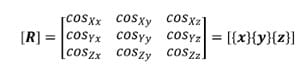
where {x}, {y}, and {z} represent the column vectors of the local axis x,y and z respectively.
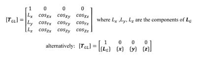
The transformation matrix [TGL] describing the location and orientation of the local coordinate system with respect to the global system is composed of both the position vector of the local origin LG and the rotation matrix [R] along with a placeholder row for mathematical convenience. The transformation matrix is written as follows:
The location of a point PL expressed as coordinates in the local reference frame can be transformed into coordinates in the global reference frame PG using the following property of the transformation matrix:
{PG} =[TGL]{PL}
where {PG} and {PL} represent the point in the global and local systems respectively.
Likewise, the components of any vector VL in the local reference frame can be transformed into components in the global reference frame VG by the following property of the rotation matrix:
{VG}=[RGL]{VL}
where {VG} and {VL} represent the vector in the global and local systems respectively

Figure 10: Local to Global Transformations
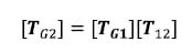
Similarly, the transformation matrix between two local reference frames [T12], position two with respect to position one, can be calculated from the two transformation matrices defining each system in the global reference frame [TG1] and [TG2]. Any position of a local system with respect to the global system can be viewed as a displacement from some initial position. Thus, it can be viewed as the composition of two displacements: from global to position one and from position one to position two. Stated in matrix form:
Note that the following property of transformation matrices defined with this notation convention was applied, which states that the inverse of any transformation matrix represents its physical inverse i.e. the transformation considering the opposite reference frame fixed.
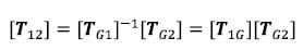

Figure 11: Local to Local Transformations
5.2.2 Euler Angles
The following is a brief description of Euler Angles. All notation conventions are taken from Zatsiorsky (Zatsiorsky). Any rotation in three-dimensional space can be expressed as three sequential rotations: the first about a global fixed axis, the second about an axis of the once-moved reference frame, and the third about an axis of the twice-moved reference frame. The Euler angles are also referred to as yaw, pitch and roll. In common terminology for airplanes, yaw is defined as rotation about the vertical global axis i.e. with respect to the ground. Pitch is defined as rotation of the plane about an axis through the wings of the plane i.e. nose up or nose down. Finally, roll is defined as rotation about the long axis of the plane running from tail to tip. The following notation will be used to describe rotation about the global X, followed by the moved y and twice moved z axes: Xy’z”. Note that the number of (‘)’s corresponds to the number of preceding rotations and that there are 12 possible Euler sequences, six of which are permutations of the order xyz. Finite rotations in three-dimensional space are not commutative; thus each rotation sequence is unique. Euler angles can be expressed as elements of the rotation matrix [R]. For the rotation sequence Xy’z” with sequential rotation angles &# 945; , &# 946;, and &# 933;, the rotation matrix expressed as a function of the sequential rotations is calculated as follows:
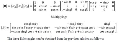
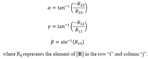
The three Euler angles corresponding to any of the other sequences can be calculated in a similar manner. The selection of the most appropriate Euler angle sequence as it pertains to spine biomechanics has been much debated, and no standard has been established. The order flexion/extension followed by axial rotation followed by lateral bending has been used by Panjabi, Goel and others while some investigators have taken the average of all six possible Euler angle permutations (Crawford, Yamaguchi et al. 1996). In addition, the order of primary motion followed by secondary coupled motions for a given mode of loading has been used (Nowinski, Visarius et al.). Crawford has shown that the conclusion drawn from experimental data regarding the coupling of lateral bending and axial rotation in the cervical human spine can be different depending on which permutation of rotations is used to calculate the Euler angles describing joint motion. He therefore proposed the sequence axial rotation followed by lateral bending followed by flexion/extension based on an argument from symmetry (Crawford, Yamaguchi et al. 1996). Given the lack of standardization on the Euler angle sequence used in spine biomechanics, the sequence Xy’z”, corresponding to flexion/extension, followed by lateral bending, followed by axial rotation was accepted based on the rationale that the Flexion/extension ROM in the human spine is in general the greatest of the three modes of motion. Additionally, no attempts at quantifying rotation coupling will be made based on the Euler angles calculated.

Figure 12: Illustration of Euler Angles
5.3 ROM RESULTS
By the methods outlined above, a time series of rigid body
transformations [TGAi]t for each vertebral body i was calculated based on the time series of locations of the associated digitized fiducials. The relative transformation between each body and the one directly inferior to it [TA(i-1)Ai]t for each time t was then calculated as follows.

Figure 13: Representative Euler Angle Plot
The ROM of each FSU for each of the twelve specimens was calculated as the difference between the maximum and the minimum value of the associated Euler angle for each mode of loading. Flexion/extension corresponds to a. Lateral bending corresponds to &# 946;, and axial rotation corresponds to &# 933;. The results for each mode of loading are presented in Tables 1-3 below. The results are reported in terms of the mean and standard deviation of the ROM at each level.

Table 1: Flexion Extension ROM Results

Table 2: Lateral Bending ROM Results

Table 3: Axial Torsion ROM Results
Six of the spines used in this study were instrumented with pedicle screw fixation at the L4-L5 level as well as interference facet fixation screws at the L2-L3 level. Prior to implantation each specimen was destabilized by performing a laminotomy and a partial facetectomy. The specimens were then tested in this condition followed by instrumentation as described above and subsequent testing. A one-way, repeated measures ANOVA with Bonferroni correction for multiple comparisons was conducted to detect differences in the ROM based on the condition of the spine. A significant difference was found in the flexion/extension ROM between the Intact and Instrumented conditions (p=0.027) and between the Destabilized and Instrumented conditions (p=0.004) for the FSUs instrumented with pedicle screw fixation. The ROM between Intact and Destabilized conditions was not found to be statistically different (p=0.135).

Table 4: Intact Flexion/extension ROM Results

Table 5: Destabilized Flexion/extension ROM Results

Table 6: Fixation Flexion/extension ROM Results
5.4 CALCULATION OF THE HELICAL AXIS OF MOTION
According to Chasles’ Theorem, any motion of a rigid body can be described as a rotation about a particular axis, known as the helical or screw axis, and a translation along that axis (Zatsiorsky). This graphical representation of rigid body kinematics is much easier to conceptualize than rigid body transformation matrices. Figure 14 shows a rigid body represented as a gray box rotated about an axis in three-dimensional space. In addition, the position and According to Chasles’ Theorem, any motion of a rigid body can be described as a rotation about a particular axis, known as the helical or screw axis, and a translation along that axis (Zatsiorsky). This graphical representation of rigid body kinematics is much easier to conceptualize than rigid body transformation matrices. Figure 14 shows a rigid body represented as a gray box rotated about an axis in three-dimensional space. In addition, the position and

Figure 14: Helical Axis of Motion
In practice, the helical axis is calculated from a single, finite displacement, giving rise to the term finite helical axis. Calculation of the finite helical axis parameters is subject to conflicting stochastic as well as deterministic errors which are inversely and directly proportional to finite rotation magnitude respectively (Woltring, Huiskes et al.). Stated alternatively, small increments of rotation are required to appropriately describe the continuous motion of the rigid body, but large stochastic errors result if the increment is not sufficiently large. In light of these considerations, an algorithm was developed to calculate the location of the helical axis of motion (HAM) for a user-defined increment of rotation. The helical axis parameters were extracted from the rigid body transformation matrices by the method given by Spoor and Veldpaus (Spoor and Veldpaus). The algorithm was validated by collecting kinematic data from rigid body flags fixed to a typical door hinge shown in Figure 16. The true axis of rotation was approximated by digitizing two points on the hinge. The hinge was then moved manually through several cycles of approximately 90° while the rigid body flag marker positions were tracked. The HAM parameters were then calculated by the algorithm below.
5.4.1 Calculation Algorithm
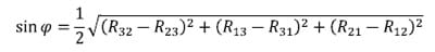
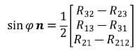
The helical axis parameters were calculated using the following method described by Spoor and Veldpaus (Spoor and Veldpaus). As described above, the motion of a rigid body between position 1 and position 2 can be characterized by a rotation matrix [R] and a translation vector. In the following description, the translation vector will be denoted, v. The motion can also be described as rotation through and angle f about the helical axis and a translation t along the axis. The unit vector along the helical axis will be denoted by n, and s will be the position vector of a point on the helical axis such that s and n are orthogonal. The angle f can be calculated using the following equation:
Once the angle f is known, the unit vector n can be calculated by solving the following equation:
The vector v can be taken directly from the transformation matrix describing the motion from position 1 to position 2. Using the vector v and the calculated vector n, the magnitude of the translation t along the helical axis can be calculated as follows:

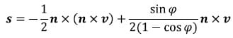
The position vector s of a point on the helical axis can be calculated from n, v and f from the following equation:
Once the parameters of the helical axis are known, it is possible to calculate the intersection of the helical axis with any plane. Figure 15 illustrates the intersection, represented as a red dot, of the helical axis n with a plane orthogonal to the x coordinate axis. For flexion/extension motions for example, it is interesting to know the intersection of the helical axis with the plane perpendicular to the anatomical x axis. In the following description, the radius vector of the point P will represent the location of the intersection of the helical axis with the plane normal to the x axis, n will represent the helical axis, and s will denote the position vector of a point on the axis as defined above. It is possible to express t
he point P in terms of the vectors s and n and a scalar q:

Since P lies in the plane of interest, it is by definition perpendicular to the normal vector defining the plane, in this case x. The scalar q and thus the vector P can be found as follows:
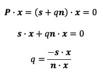

Figure 15: Illustration of Axis Plane Intersection
5.4.2 Validation Procedure and Results The HAM calculation algorithm was validated by calculating the helical axis for an object with a known axis of rotation, a typical door hinge. Two rigid body flags were fixed rigidly to either face of the hinge as shown in Figure 16. Prior to testing the axis of rotation of the hinge was approximated by digitizing two points on the hinge axis. The flag orientations were tracked using the Optotrak while the hinge was manually opened and closed. The HAMs were calculated based on an angular step size of 0.5°. Figure 17 shows the calculated HAMs as thin, multicolored lines along with the approximated axis of rotation as the thick, black line defined by the two digitized points. Figure 18 shows the points of intersection of each calculated HAM with the plane perpendicular to the approximate axis of rotation. The intersection point error, defined as the distance from each point to the intersection of the approximated axis of rotation, was calculated as 1.10mm ± 1.27mm (mean ± standard deviation). Additionally, the orientation error, defined as the angle between the calculated axes and the approximated axis, was calculated as 2.87°±3.15°. These error statistics are similar to those reported by others (Zhu, Larson et al.),(Chèze, Fregly et al.),(Rousseau, Bradford et al.).

Figure 16: Instrumented Hinge

Figure 17: Calculated HAM vs. Known Axis of Rotation

Figure 18: HAM Orthogonal Plane Intersections
5.5 HAM RESULTS
As stated above, the error associated with the calculation of the HAM is related to the angular step size used in the calculation. Therefore, in order to report consistent results, it is necessary to calculate all axes above some threshold value for which the error has been bounded. Ideally, all helical axes would be calculated based on the same angular step size, however, this is impractical in spine research as each specimen will have a unique ROM and it is convenient to have the same number of helical axes calculated for each specimen and mode of loading for the purpose of comparison. Since error was characterized for a step size of 0.5° and 3° is a conservatively small estimate for the range of motion of any FSU for any given mode of loading, it was decided that six axes would be calculated between peak flexion/extension, left and right lateral bending and left and right axial rotation. So that each HAM would be calculated at the same time for each FSU, the time frames at which the axes would be calculated were generated based on the superior motor displacements instead of individual FSU angular displacements. Figure 19 shows the superior motor displacement vs. time, the blue line, along with the points in time between which the HAM parameters were calculated, indicated by the asterisks, for one of the specimens. Note that there are 11 time frames in all corresponding to 10 sets of HAM parameters, one between each pair of time frames. Figure 20 shows the HAMs calculated for the axial rotation test of one specimen along with their intersections with the XY plane of the anatomical coordinate system of the inferior vertebral body of a single FSU. Note that the HAMs are plotted in three dimensions and that the XY plane is described by the grid lines indicating zero on the Z axis.

Figure 19: Time Frames Indicating Endpoints of HAM Calculations

Figure 20: XY Plane Intersections for a Single FSU during Axial Torsion
Figure 21 displays the helical axes, shown in yellow, calculated at each FSU for a single specimen during the flexion/extension test superimposed on the three-dimensional model of the vertebral bodies. In addition, the orientation of the x axis for each FSU local coordinate system is shown in blue which represents the expected orientation of the HAM for flexion/extension motion. Note that the orientation of the axes along the medial/lateral axis corresponds to what is expected from flexion/extension motion and what is reported in the literature (Zhu, Larson et al.). Still, it should be noted that there is some obvious deviation in the helical axes from the actual medial/lateral axis which may have ramifications regarding the interpretation of the two-dimensional center of rotation often calculated from planar radiographs under the assumption that the axis of rotation is orthogonal to the plane of measurement.

Figure 21: Helical Axes During Flexion/extension
Figures 22, 23 and 24 display the normalized HAM plane intersections for each FSU averaged across all six specimens superimposed on a single normalized FSU. The HAM plane intersections for each FSU were normalized with respect to the width of the inferior vertebral body of the FSU defined by the distance between the lateral most fiducials. The model of a single FSU was normalized by the same parameter and is shown in the following figures. Note that in all three figures, yellow corresponds to L1-L2, blue corresponds to L2-L3, green corresponds to L3-L4 and red corresponds to L4-L5. The 10 dots shown for each level correspond to the 10 calculated HAMs.

Figure 22: Mean HAM Intersections for Flexion/extension

Figure 23: Mean HAM Intersections during Lateral Bending

Figure 24: Mean HAM Intersections during Axial Torsion
A one-way, repeated measures ANOVA with Bonferroni correction for multiple comparisons was conducted to establish if there was any significant difference in HAM intersection locations between levels. This analysis revealed that there was a significant difference between the normalized mean HAM intersection locations at various levels during flexion/extension. The mean of the 10 ca
lculated HAM intersections were significantly different between L1-L2 and L3-L4 (p=0.024), L1-L2 and L4-L5 (p=0.013), and between L2-L3 and L4-L5 (p=0.011). In addition, the anterior/posterior position of the HAM intersections averaged across specimens was found to be significantly different in flexion compared to Extension at the L1-L2 level (p=003). Figure 25 shows the HAM intersections averaged across all specimens and time frames as the solid dots along with the HAM intersection corresponding to peak flexion, indicated by the open squares, and peak extension, indicated by the open triangles, superimposed on the same semitransparent, normalized FSU as the previous figures. The colors indicate level as they did in the previous figures (yellow=L1-L2, blue=L2-L3, green=L3-L4, red=L4-L5). Figures 26 and 27 present the same data for the lateral bending and axial rotation tests respectively. The open squares indicate peak right lateral bending and peak right axial torsion, while the open triangles indicate peak left lateral bending and axial torsion.

Figure 25: Mean HAM Intersections

Figure 26: Mean HAM Intersections
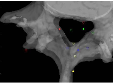
Figure 27: Mean HAM Intersections
5.6 INVESTIGATION OF VISCOELASTICITY
5.6.1 Definition of appropriate parameters
Several parameters have been used to characterize the viscoelastic properties of the ligamentous spine including the NZ and corresponding Elastic Zone (EZ), the Lax Zone (LZ), linear elastic stiffness and hysteresis area (Panjabi 1992), (Crawford, Peles et al.), (Gardner-Morse and Stokes). The NZ is defined as the part of the physiologic ROM in which intervertebral motions are produced with minimal internal resistance. The EZ is defined as the remaining portion of the ROM measured from the end of the NZ to the physiologic limit (Panjabi 1992). The NZ has been measured using various test procedures, and experimental results suggest that it is a more sensitive parameter for evaluating spinal instability than ROM (Panjabi 1992). Panjabi developed a process of in vitro testing utilizing pure moments applied in discrete, incremental steps up to the estimated physiological limit for three load cycles. He defined the NZ as the residual displacements between the beginning of the third load cycle in one direction and the same load cycle in the opposite direction (Panjabi 1992). It is not immediately clear what this measurement corresponds to in the case of continuous sinusoidal load cycling, but some researchers have defined the NZ in this loading modality as the zone between the two intersections of the hysteresis loop and the axis representing zero load as shown in Figure 28 (Phillips, Tzermiadianos et al. 2009). It is not apparent that this calculation corresponds to the NZ as outlined by Panjabi, and it is expected to be a function of the loading rate as well as the viscoelastic properties of the spine. Thus it is not repeatable among testing laboratories using differing testing apparatus and loading parameters. The hysteresis area is defined as the area bounded by the hysteresis loop for one load cycle and represents the amount of energy dissipated by the specimen during the cycle. This energy dissipation has been shown to be a sensitive parameter in the evaluation of spinal fixation devices (Deguchi, Cheng et al.). While this parameter is also expected to be a function of the loading rate, its physical interpretation is clear, and its calculation by numerical integration of the test data requires no definition of arbitrary parameters as required by the Lax Zone and linear elastic stiffness.

Figure 28: Representative Hysteresis Loop
5.7 APPROXIMATION OF HYSTERESIS AREA
5.7.1 Algorithm
The hysteresis loop is a plot of displacement vs. load throughout a given test and is used to help characterize the viscoelastic properties of the specimen. An algorithm was developed to approximate the area bounded by the hysteresis loop generated during each test. The most significant challenge in developing such an algorithm is in dealing with noisy data which exists in the region near zero load. This noise is attributable to the relative laxity of the spine near its neutral position which inhibits the smooth control of motor displacements. Due to the noisy nature of the data encountered, it was decided that an algorithm based on polynomial least-squares fits would be appropriate. The hysteresis loop was first separated into two parts: an “upper” and a “lower” curve. A tenth-order polynomial was then fit to each curve and the area between the two was calculated by evaluating the integral of the difference between the two polynomials over the range of the hysteresis loop. The validity of the polynomial integration algorithm was checked against hand calculation of a single set of polynomial integrals. The 10th order polynomial was selected because it was the lowest order to converge to an accuracy of 10-2 J in specimens tested previously in the laboratory.
5.8 HYSTERESIS AREA RESULTS
Figure 29 shows the hysteresis plot for a single level of a specimen. The green and blue data points represent the data separated into upper and lower curves respectively. The solid, black lines represent the polynomial fit to each curve. The calculated hysteresis area is the area bounded by the black lines on the interval between the minimum and maximum displacement values of the experimental data. Tables 4-6 display the hysteresis area results for each FSU averaged across all twelve specimen in both absolute terms and in terms of the percentage contribution to total energy dissipated, defined as the sum of the value for all the levels. A one-way, repeated measures ANOVA with Bonferroni correction for multiple comparisons was conducted to detect differences in the area calculations based on the mode of loading. Significant differences were found at every FSU between every mode of loading for the energy dissipated by the spine. The energy dissipated by the spine is significantly greater in flexion/extension than in lateral bending and also significantly greater in lateral bending than in axial rotation even though the impulse or the time history of force imparted on the spine is the same in all three tests.

Figure 29: Example Hysteresis Plot with Polynomial Fits

Table 7: Flexion/extension Hysteresis Area Results

Table 8: Lateral Bending Hysteresis Area Results

Table 9: Torsion Hysteresis Area Results
In the same study mentioned above regarding evaluating the destabilized and pedicle screw fixed conditions, the hysteresis area was calculated for each conditio
n. Tables 10-12 contain the calculated areas for the three treatment cases. A one-way, repeated measures ANOVA with Bonferroni correction for multiple comparisons was conducted to detect differences in the area calculations based on the condition of the spine. The only statistically significant difference in flexion/extension hysteresis area was between the Destabilized and Instrumented conditions (p=0.015).

Table 10: Intact Flexion/extension Hysteresis Results

Table 11: Destabilized Flexion/extension Hysteresis Area Results

Table 12: Fixation Flexion/extension Results
6.0 INVESTIGATION OF FACET ARTICULATION
The transfer of load across the facet joint has been measured using both strain gages and pressure sensitive film (Kahmann, Buttermann et al.),(Lorenz, Patwardhan et al.). Lorenz et al. were able to investigate facet normal loads and contact areas using Fuji Prescale pressure sensitive film, a Fuji Prescale Densitometer and a film scanning device. The group investigated the facet normal load and contact area under progressively larger applied axial loads with the FSU in neutral and extended positions. The group was able to show that facet normal loads were higher in extension than in neutral postion at both the L2-L3 and L4-L5 levels. Additionally, they showed that the contact area moved cranially at L2-L3 and caudally at L4-L5 with increasing applied compressive loads while the FSU was in extension. The use of pressure sensitive film is inherently invasive since it requires incision of the facet capsule and insertion of a piece of film between the articulating surfaces which would undermine the primary directive of characterizing the kinematic response of the intact lumbar spine.
Kahmann et al. investigated the effects of facet capsulectomy and discectomy on facet load and resultant load location using four strain gauges bonded to the cranial articular process opposite the facet surface. The group was able to show that there was a caudal shift in resultant load position with discectomy and that capsulectomy had a variable effect on load position. While the strain-gauge-based method used by Kahmann et al. does not disturb the facet capsule, it requires significant instrumentation of each specimen and does not provide easily interpretable visualization techniques.
The goal of the testing procedure developed is to derive a noninvasive representation of facet articulation based on the application of acquired kinematic test data to a CT-based solid model of the spinal segment. Below, the fundamental steps of the procedure are described in detail.
6.1 DEVELOPMENT OF TEST ALGORITHM
6.1.1 Development of Rigid Body Model
Commercially available image segmentation software (ScanIP, Simpleware UK) was used to generate three-dimensional models of each vertebral body within each lumbar segment from CT scans with voxel size 0.625mm x 0.270mm x 0.270mm obtained from a GE Medical Systems 4-Slice Lightspeed scanner. The vertebral bodies were segmented based on pixel intensity, and a morphological closing filter was used to fill in the trabeculae so that each vertebral body was modeled as a solid volume. The aluminum fiducials were segmented in a similar manner. The segmentation process is displayed in Figure 30 which displays a screenshot of the segmentation software after segmentation of the L1 and L2 bodies of one specimen. The upper and lower left and upper right sections show the CT scan reconstruction in three orthogonal views: axial, sagittal and coronal respectively. The lower right view displays a three-dimensional reconstruction of the vertebral body models. Note that the differing colors represent two different solid models.
The solid models generated from CT segmentation were exported in stereolithography (STL) format. STL files define surfaces by triads of vertices defining triangular faces along with outward-facing surface normal vectors for each face. Figure 31 displays a surface defined by the vertices, shown in red, and associated normal vectors, displayed in yellow. Each facet is rendered in blue with edges in black. A custom MATLAB function (STL2cloud_unique.m) was written to import the solid model data into the MATLAB workspace. This function scans the text of the ASCII STL file and saves the vertex and normal vector data in appropriately formatted arrays. In order to minimize memory and computational requirements, repeated vertices inherent to STL format were not saved. Using a built-in MATLAB function, the unique points defining each model were extracted along with an array of indices that could be used to reconstruct the full set of data including the repeated vertices which are required for rendering of the model. The model of L1-L5 rendered in the MATLAB environment is displayed in Figure 32. Note that every vertebral body is rendered in a different color signifying that each one is defined as a separate body.

Figure 30: Image Segmentation and Reconstruction of L1 and L2 Models

Figure 31: STL Surface Definition

Figure 32: Lumbar Segment in MATLAB Environment
6.1.2 Defining the Region of Interest
The Region of Interest (ROI) is defined as the articular surface of the facet. This region will be defined as those surfaces within a threshold distance from the surface of the neighboring vertebral body. Since information regarding the articular cartilage is not present in the CT data, some assumptions will be made regarding the cartilage layer. While data has not been found in the literature regarding facet cartilage thickness in the lumbar vertebrae, a mean maximum thickness of approximately 1mm has been reported for the cervical spine (Womack, Woldtvedt et al.),(Yoganandan, Knowles et al.). Based on these findings a threshold of 3mm was established for defining the ROI based on the rationale that each surface can conservatively be expected to have a uniform, 1mm thick layer of cartilage and that in the neutral position a conservative estimate for the gap between any portions of the articular surfaces is 1mm. Using built-in and custom built functions, a program (AutoSelect.m) was written to automatically select the ROI on each vertebral body based on the 3mm distance criterion and save the indices of those vertices defining the ROI for subsequent use. Figure 33 shows the ROI representing the left facet articular surfaces for a single FSU. Each triangular face on each surface is colored based on the distances of the three vertices defining it to their nearest neighboring points on the adjacent surface. Note that dimension on the color bar are in millimeters and that dark blue corresponds to 0mm while red corresponds to 3mm. Figure 34 shows the ROI distance map superimposed on semi-transparent vertebral bodies of a single FSU. This color map illustrating the nearest neighbor distances of the ROI vertices will hereafter be r
eferred to as the Vertex Distance Map (VDM).

Figure 33: Left ROI for Single FSU

Figure 34: ROI Distance Map Superimposed On Transparent Vertebral Bodies
6.1.3 Application of Test Kinematics to Rigid Body Model
6.1.3.1 Registration
In order to apply the acquired kinematic data to the 3D model, the location of at least three non-collinear points on each vertebral body must be known in both the image reference frame and the Optotrak reference frame. In a preliminary study of six lumbar specimens an attempt was made to circumvent the well known effects of metal artifact on CT images by using a doped agar preparation as a fiducial. Unfortunately, some problems are associated with this procedure. First, it is difficult to ensure that the agar conforms to the surface of the hole drilled into the bone; since it is this surface that is subsequently used to digitize the point using the marker probe, significant registration error can result. Second, it is difficult to consistently mix and apply the agar to the specimen resulting in inconsistent shape and intensity of the fiducials. In light of these shortcomings, a method of inserting 3mm aluminum balls into the specimen was developed. The use of aluminum fiducials resulted in no visually apparent metal artifact, as shown in Figure 35, due to the low density of the material. In addition, a custom tip with a cupped end for the marker probe was designed to fit over each spherical fiducial and digitize its centroid. Figure 36 shows the four-marker probe in use digitizing a fiducial on the body L3 in the reference frame of the rigid body flag labeled “2”. Figure 37 shows the solid models of segmented fiducials, shown in red, superimposed on the model of the corresponding vertebral bodies for one FSU. Eight of the original 12 specimens were tested using this new technique. Only seven of those eight were used in the analysis of the data because of the severe degeneration of one of the specimens as outlined in Discussion.

Figure 35: Aluminum Fiducial Results in Low Artifact in CT

Figure 36: Fiducial Digitization

Figure 37: Fiducial Segmentation
The centroid of each fiducial in the image reference frame was calculated as the mean location of the vertices defining the fiducial surface. Local coordinate systems for each vertebral body were defined based on the fiducial centroids by the same method shown in Figure 9 and will be referred to as local image reference frames. The corresponding transformation matrices will be expressed as [TIBi] for each body Bi. The location of each vertex PBi in the local image reference frame for each body was calculated as follows:
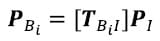 >
>where P1 represents the location of the vertex on the global image reference frame
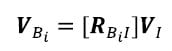
Similarly the orientation of each face normal vector was transformed into the local reference frame as follows:
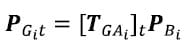
The assumption of registration is that the fiducials remain fixed with respect to the vertebral bodies between CT scanning and digitization. Therefore, the locations of points defining the surface of the vertebral body with respect to the reference frame based on the fiducials are the same in the local image reference frame and the local anatomic reference frame derived from fiducial digitization. Therefore, the location of any point on the surface of a vertebral body in the global Optotrak reference frame can be calculated using the global to anatomical transformations [TGAi] calculated from the digitized fiducial locations as follows:
 >
>As outlined above a time series of global to anatomic transformations [TGAi]t was derived from the data collected by the Optotrak. The position of the points defining the surfaces of each vertebral body i at any time frame t of the test is then easily calculated. Surface normal vectors are calculated in a similar manner using the rotation matrix.
Due to computational limitations, the surface definition for each vertebral body was only calculated at the time frames used to calculate the helical axes of motion. This was done convenience of comparison between HAM locations and facet articulation parameters. At each of these time frames, all vertices and normal vectors were transformed based on the kinematic transforms derived from the Optotrak data. In addition, the nearest neighbor point distances were recalculated for each point in the ROI. The updated surfaces and distance maps were then rendered and captured as a video frame.
6.1.3.2 Registration Error
The registration error can be quantified as the disparity between the fiducials in each corresponding local image and anatomical reference frame. The mean error calculated for each vertebral body in each of the seven specimens used in this study was 1.69mm with a standard deviation of 0.50mm. A major source of error is the procedural difficulty of using the digitizing probe. In order to digitize a point, at least three of the four markers on the probe must be visible, which is difficult to achieve while maintaining full contact of the cupped tip to the spherical fiducial for some of the fiducials, particularly those located on the lamina. Additionally, deformation of the underlying tissue during digitization itself contributes to registration error. Furthermore, the tip offset or location of the pointer tip with respect to the ILED markers was calculated using the manufacturers pivoting algorithm with an RMS error convergence criterion of 0.4 mm indicating the approximate accuracy of the probe itself. Uncertainty about the location of facet surfaces of a magnitude of 1mm or greater on average renders interpretation of the VDM impossible.
This uncertainty can be removed if the assumption is made that the relative orientations of the vertebral bodies in the scan position and the initial, zero-load condition at the beginning of each test are the same. Based on this assumption, a correction transformation can be calculated for each vertebral body.
This is a reasonable assumption since the specimen is under essentially zero load in each condition. In order to test this hypothesis, three specimens were thawed and instrumented with rigid body flags. The relative locations of the flags were then recorded as the specimen laid on the table in the same orientation as during CT scanning. Each specimen was then loaded into the machine, and all loads were set to zero as is done prior to testing. The relative position of each flag was again recorded. The difference between the relative flag orientations in the two conditions for each of the 12 FSU’s was then calculated in terms of a single rotation about a helical axis. The average magnitude of this angle was 0.618° which corresponds to 6.31% of the average range of motion for the specimens tested and 7
.00% of the average range of motion of all specimens in this study. The average difference in the distances between adjacent flag coordinate system origins was 0.86 mm.
Note that the correction transformations are calculated from the first frame of the flexion/extension test only since this is the first test conducted for each specimen. The initial position assumption is not expected to hold after the specimen has been loaded. The same set of correction transformations is then applied to the kinematic transformations for each time frame of each test. The correction transformations, representing offsets between reference frames based on the digitized fiducials and reference frames based on the fiducials in CT, are calculated as follows. First, the transformation for each vertebral body in both the Optotrak and Image reference frames with respect to the inferior most body is calculated. It is assumed that this fixed reference frame in the Optotrak and Image reference frames are synonymous and will be denoted by C.
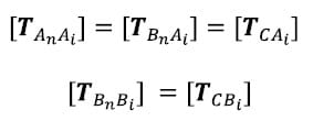
where An and Bn represent the inferior most body in the Optotrak and Image reference frames respectively. Now the positions of each vertebral body from the Image reference frame and from the Optotrak reference frame at time 1 are expressed in the same fixed reference frame and will be referred to as the Image and Optotrak bodies respectively. The initial position assumption is that these two bodies converge at time frame 1:

The correction transformation is one describing the position of each Image body with respect to its corresponding Optotrak body.
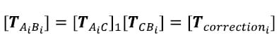
The corrected Optotrak body transformations or the transformations describing each vertebral body with respect to the inferior most body can now be calculated at each time frame by multiplying the kinematic transformations at each time frame by the correction transformation for the corresponding vertebral body:
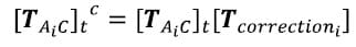
To verify the algebra, the application of the correction transformation at time frame one results in restatement of the initial position assumption:

6.1.4 Interference Detection
An interference detection algorithm was written and applied to the ROI. The algorithm is based upon the projection of each vertex of one surface (the “vertex search” surface) onto the normal vector, oriented outward, of the associated nearest face of the adjacent surface (the “face search” surface). Once each vertex of the first surface is associated with its nearest face on the apposing surface, the dot product of a vector defined by the vertex and the centroid of the nearest face and the normal vector of that face is evaluated. If the value of the dot product is negative, then interference has occurred and the vertex is displayed on the screen. Figure 38 shows the results of interference detection between two obviously intersecting surfaces. The blue surface corresponds to the “vertex search” surface while the green surface corresponds to the “face search” surface. The vertices that the interference algorithm has determined to be on the inside the opposite surface are shown in white. This serves as verification of the interference detection algorithm. This parameter may serve useful for indicating facet force transmission if sufficient certainty can be obtained regarding facet surface locations. While surface interference was calculated for each of the specimens in this study, no analysis was applied using this parameter.

Figure 38: Interference Detection
6.2 DELINEATION OF APPROPRIATE PARAMETERS
The VDM is easy to interpret visually in that blue regions indicate areas of intimate contact while areas more to the red end of the spectrum do not. It is apparent from viewing the VDM videos that the interaction of the facet surfaces changes significantly over the course of the range of motion. One also notices that there is significant variability between specimens as to the
extent of facet “contact” signified by blue regions and the timing and location of the contact for the same tests. While the visual interpretation of the VDM gives an intuitive sense of what is happening at the facet on a case-by-case basis, quantifying that same data mathematically is much more difficult. One metric that might mirror the visual interpretation of the data is the ratio of “blue” to “red” regions on the VDM. This can be estimated by selecting some threshold and calculating the number of faces defining the ROI with distances below that threshold at each time frame. This metric will be expressed at a ratio of the total number of faces defining the ROI and will be referred to as the Contact Area Ratio (CAR). It should be noted that this is an approximation since it is assumed that each face defining the facet surfaces is the same size, which one would expect from the fairly uniform meshing of the segmentation software and appears to be approximately true based on visual inspection. Based on the assumptions outlined above regarding the selection of the ROI, a CAR threshold of 2mm was selected. Essentially, it is assumed that each facet surface has a 1mm thick layer of cartilage upon the subchondral bone and any two surfaces within 2mm are thus in contact.
6.3 RESULTS
The CAR was calculated at each of the time frames for which the HAM parameters were calculated for the same seven specimens. Figure 39 shows the CAR for each FSU averaged across the specimens at each of the time points for the flexion/extension test. Note that there are eight lines representing the eight articular surfaces of the four FSU’s in each specimen. The thick, blue line represents the average CAR across all FSU’s and specimens for the flexion/extension test. Note that time frames three and nine corresponds to peak flexion and peak Extension respectively. From the graph it seems apparent that for each FSU, the CAR increases going from flexion to extension. A two-way, repeated measures ANOVA with Bonferroni correction for multiple comparisons was conducted to detect differences in CAR between full flexion and full extension. Indeed there is a significant difference between the CAR for each FSU averaged across all specimens at of the time frames three and nine, corresponding to full flexion and full extension respectively. These findings indicate that the contact area of the facet is greater in Extension than in flexion which corresponds directly to what is perceived from visual interpretation of the VDM video. It seems from these results that the role of the facet is to serve as a stop in Extension. These results are also in accordance with data reported by Lorenz et al. that under low axial loads, the total facet contact area is greater during extension than in neutral position for both L2-L3 and L4-L5 levels (Lorenz, Patwardhan et al.).

Figure 39: Mean Contact Area Ratio For Flexion/extension
7.0 DISCUSSION
For both the calculation of the HAM and the model-based method, only seven of the original 12 specimens were studied. Four specimens were tested using the gel fiducial method outlined in the Registration section above before the aluminum fiducial method was developed. Of the remaining eight, one of the specimens, shown in the le
ft of Figure 40, was excluded from HAM and CAR data analysis. It was concluded that this specimen would be excluded from any treatment-related biomechanical tests due to clear radiographic pathology, a standard metric for specimen selection. In addition, the ROM at three of the specimen’s FSU’s were below 1.5° precluding the calculation of accurate HAMs for the specimen. Figure 40 illustrates the range of specimen variability encountered in spine research with the aforementioned degenerated spine on the left and a very healthy specimen on the right. Obviously this biologic variability introduces difficulty into characterizing the “normal” spine. It is therefore recommended that future studies involve some form of clinical evaluation prior to testing so that the metrics presented here can be used to evaluate healthy vs. pathologic spine biomechanics.

Figure 40: Example of Specimen Variability
7.1 SUMMARY
It has been shown, as expected, that ROM is a sensitive parameter in evaluating spinal fixation. Additionally, it has been shown that hysteresis area, or the energy absorbed by the specimen during a complete cycle of testing, is not as sensitive as ROM in evaluating rigid fixation. It is still hoped that this parameter will be useful in evaluating motion preservation devices because of its simplicity in calculation and its physical interpretation. Additionally, it was shown that the energy dissipated during flexion/extension was greater than that in lateral bending, which was greater than that in axial rotation for a constant quantity of energy input in all three cases. This implies that the osteoligamentous structures of the spine are capable of dissipating more energy, and thus absorbing more impact, in flexion/extension than in the other modes of loading which may have implications with regard to injury prevention and analysis. It is interesting to note that the energy dissipated by the severely degenerated specimen, shown in Figure 41, was remarkably symmetric in the three modes of loading with values in flexion/extension, lateral bending and axial rotation of 23.82, 23.93, and 24.16 compared to the corresponding mean across all specimens of 90.18, 48.49, and 21.07. These results make physiologic sense as the viscoelastic, asymmetrical, intervertebral disk gives way to the less viscoelastic bone, one would expect a lower magnitude of energy dissipation with a more symmetric distribution.
The HAM has been calculated by spine biomechanics researchers using various methods and constraints, such as angular step size, and has been reported several different ways, generally including an anatomical plane intersection and orientation. Due to the error characteristics of HAM calculation it is necessary to use a sufficiently large step size and preferable to calculate all HAMs based on the same step size. However, this makes comparisons regarding the location of the HAM at particular portions of the range-of-motion difficult as there could be a different number of axes among levels of the same spine. In addition, during load control tests, the proper time points for calculating the helical axes cannot be set a priori based on the load waveform. This is because the viscoelastic response to loading is variable among specimens. The solution to this dilemma presented was to calculate a conservative number of axes between the peaks of the range-of-motion at time points determined by the motor displacements. While some variability is seen in the temporal response of FSU’s within a given specimen they are fairly consistent so that the time frames used to calculate the helical axes correspond well to the flexion/extension peaks and are relatively evenly spaced with respect to angular displacement. The resulting angular step size for all specimens tested in flexion/extension ranged from 0.35° to 3.51° with an average of 1.51° and a standard deviation of 0.52°. In fact only five out of the 280 axes calculated were below the angular step size for which the error as characterized, 0.5°. The HAM plane intersections were shown to be sensitive enough to describe some difference between the kinematic responses of different levels of the lumbar spine as well as to detect changes throughout the range-of-motion at the L1-L2 level. This sensitivity lends credence to the idea that the helical axis parameters will be useful in the evaluation and in driving the design of motion preservation devices.
A noninvasive method for describing facet articulation was developed based on the application of test-derived kinematics to three-dimensional solid models of the spine. While this was done through an extensive and laborious development of custom software, the end-result in functionality and data integration was worth the cost. A full gamut of test results can be obtained from a specimen within 20 minutes of testing with minimal manual manipulation of raw data. A new parameter approximating the proportion of facet articular surface area in contact based on a discreet distance map between two opposing surfaces was presented. This parameter was shown to be sensitive enough to detect differences in facet contact area between full flexion and full extension, which is in accordance with previously published data on facet articulation (Lorenz, Patwardhan et al.). These findings may have significance in regard to Finite Element Modeling of the spine as the facets are often modeled as continuously contacting elements (Chen, Zhong et al. 2009).
7.2 FUTURE WORK
The proximate goal of future work is to investigate the lateral bending and axial rotation modes of loading more rigorously. Particularly, the orientation of the HAM can be used to quantify the degree of coupled rotation between axial rotation and lateral bending without the pitfall of order-dependence seen with Euler angle descriptions of motion. A more easily interpreted parameter describing the location of the HAM than the point of intersection with an anatomical plane during these two modes of loading should also be developed. In flexion/extension the orientation of the HAM is nearly perpendicular to the sagittal plane so the point of intersection with that plane is relatively insensitive to changes in axis angulations resulting from either altered kinematics or measurement error. This is not the case in either of the other two modes of loading as can be seen in Figure 41 which displays the HAMs for each FSU of a particular specimen during torsion. For example, a shift of the HAM from the centerline of the vertebral body towards the right facet could result in a transverse plane intersection shift in the opposite direction. In short, the interpretation of helical axis intersection points in a plane that is not approximately orthogonal to the axis of rotation is not straightforward. Perhaps the nearest distance between the HAM and some anatomical landmark which may be proposed to influence rotation and thus the location of the helical axis, such as the facets, can be investigated. This single parameter would take advantage of the three-dimensional information provided by the HAM.

Figure 41: HAMs during Axial Torsion
In addition to HAM parameters, facet articulation in lateral bending and axial rotation should be investigated using the model-based technique as well. Additional parameters to describe facet articulation should also be developed. Proposed parameters include minimum inter-surface distances, magnitude and area of surface interference and articular surface shear translations. In addition, the sensitivity of the CAR results to the contact threshold should be investigated. While the initial position assumption has been shown to be a relatively
robust approximation for the intact spine, efforts should be made to reduce registration error either through more accurate digitization techniques or the inclusion of more sophisticated registration techniques including more registration points or surfaces. This would allow for use of this method in treated spines for which the initial position assumption cannot be assumed to hold. Additionally, fiducial location should be optimized in order to reduce the likelihood of fiducial loss during device implantation.
7.3 CONCLUSIONS
In vitro spine biomechanics testing is an integral part of spinal implant design and analysis. A paradigm shift in the clinical treatment philosophy regarding back pain, centered on concerns regarding the effect of rigid fixation on the surrounding tissues, has changed the design parameters for spinal implants. Parameters used to evaluate these new devices must expand in tandem with the more complex goal of achieving physiologic motion after implantation. The parameter (ROM) most suited for the evaluation of the binary evaluation of fusion devices, fixation vs. non-fixation, while necessary in the evaluation of motion-preserving devices, is not sufficient. A more descriptive set of parameters (HAM) were reported here with particular interest on proper and intuitive representation. In light of the sensitivity these parameters have shown to differing kinematics between specimens, it is hoped that they will be sufficient to evaluate pre and post-treatment specimens.
A method has been described here that is capable of investigating the behavior of the intact facet joint without invading the joint space or surrounding tissue. This method has been shown sensitive enough to detect changes in facet articulation throughout the range-of-motion of the intact specimen. Extrapolating from this, it is hoped that this method will be able to detect changes in facet articulation between intact and instrumented specimens.
See PDF for APPENDIX A
See PDF for APPENDIX B
BIBLIOGRAPHY
- (2008). “Optotrak Certus Motion Capture System: Technical Specifications.” Retrieved 3/2/2009, 2009, from https://www.ndigital.com/lifesciences/certus-techspecs.php.
- Chen, S.-H., Z.-C. Zhong, et al. (2009). “Biomechanical comparison between lumbar disc arthroplasty and fusion.” Medical Engineering & Physics 31(2): 244-253.
- Chèze, L., B. J. Fregly, et al. (1998). “Determination of joint functional axes from noisy marker data using the finite helical axis.” Human Movement Science 17(1): 1-15.
- Cholewicki, J., J. J. Crisco, 3rd, et al. (1996). “Effects of posture and structure on three-dimensional coupled rotations in the lumbar spine. A biomechanical analysis.” Spine 21(21): 2421-8.
- Crawford, N. R., J. D. Peles, et al. (1998). “The spinal lax zone and neutral zone: measurement techniques and parameter comparisons.” J Spinal Disord 11(5): 416-29.
- Crawford, N. R., G. T. Yamaguchi, et al. (1996). “Methods for determining spinal flexion/extension, lateral bending, and axial rotation from marker coordinate data: Analysis and refinement.” Human Movement Science 15(1): 55-78.
- Cunningham, B. W., J. D. Gordon, et al. (2003). “Biomechanical evaluation of total disc replacement arthroplasty: an in vitro human cadaveric model.” Spine 28(20): S110-7.
- Deguchi, M., B. C. Cheng, et al. (1998). “Biomechanical evaluation of translaminar facet joint fixation. A comparative study of poly-L-lactide pins, screws, and pedicle fixation.” Spine 23(12): 1307-12; discussion 1313.
- Deyo, R. A., D. Cherkin, et al. (1991). “Cost, controversy, crisis: low back pain and the health of the public.” Annu Rev Public Health 12: 141-56.
- Dvorak, J., M. M. Panjabi, et al. (1991). “Clinical validation of functional flexion-extension roentgenograms of the lumbar spine.” Spine 16(8): 943-50.
- Galbusera, F., C. M. Bellini, et al. (2008). “Design concepts in lumbar total disc arthroplasty.” Eur Spine J 17(12): 1635-50.
- Gardner-Morse, M. G. and I. A. Stokes (2004). “Structural behavior of human lumbar spinal motion segments.” J Biomech 37(2): 205-12.
- Goel, V. K., M. M. Panjabi, et al. (2006). “Test protocols for evaluation of spinal implants.” Journal of Bone & Joint Surgery – American Volume 88 Suppl 2: 103-9.
- Hazard, R. G. (2007). “Low-back and neck pain diagnosis and treatment.” Am J Phys Med Rehabil 86(1 Suppl): S59-68.
- Hilibrand, A. S. and M. Robbins (2004). “Adjacent segment degeneration and adjacent segment disease: the consequences of spinal fusion?” Spine J 4(6 Suppl): 190S-194S.
- Kahmann, R. D., G. R. Buttermann, et al. (1990). “Facet loads in the canine lumbar spine before and after disc alteration.” Spine 15(9): 971-8.
- Kalichman, L. and D. J. Hunter (2007). “Lumbar facet joint osteoarthritis: a review.” Semin Arthritis Rheum 37(2): 69-80.
- Kettler, A., F. Marin, et al. (2004). “Finite helical axes of motion are a useful tool to describe the three-dimensional in vitro kinematics of the intact, injured and stabilised spine.” European Spine Journal 13(6): 553-9.
- Lorenz, M., A. Patwardhan, et al. (1983). “Load-bearing characteristics of lumbar facets in normal and surgically altered spinal segments.” Spine 8(2): 122-30.
- Nowinski, G. P., H. Visarius, et al. (1993). “A biomechanical comparison of cervical laminaplasty and cervical laminectomy with progressive facetectomy.” Spine 18(14): 1995-2004.
- Panjabi, M. M. (1988). “Biomechanical evaluation of spinal fixation devices: I. A conceptual framework.” Spine 13(10): 1129-34.
- Panjabi, M. M. (1992). “The stabilizing system of the spine. Part I. Function, dysfunction, adaptation, and enhancement.” J Spinal Disord 5(4): 383-9; discussion 397.
- Panjabi, M. M. (1992). “The stabilizing system of the spine. Part II. Neutral zone and instability hypothesis.” J Spinal Disord 5(4): 390-6; discussion 397.
- Panjabi, M. M. (2007). “Hybrid multidirectional test method to evaluate spinal adjacent-level effects.[see comment].” Clinical Biomechanics 22(3): 257-65.
- Phillips, F. M., M. N. Tzermiadianos, et al. (2009). “Effect of the Total Facet Arthroplasty System after complete laminectomy-facetectomy on the biomechanics of implanted and adjacent segments.” Spine J 9(1): 96-102.
- Pope, M. H. (1989). “Biomechanics of the lumbar spine.” Ann Med 21(5): 347-51.
- Rousseau, M. A., D. S. Bradford, et al. (2006). “Disc arthroplasty design influences intervertebral kinematics and facet forces.” Spine J 6(3): 258-66.
- Spoor, C. W. and F. E. Veldpaus (1980). “Rigid body motion calculated from spatial co-ordinates of markers.” J Biomech 13(4): 391-3.
- Walker, B. F. (2000). “The prevalence of low back pain: a systematic review of the literature from 1966 to 1998.” J Spinal Disord 13(3): 205-17.
- Woltring, H. J., R. Huiskes, et al. (1985). “Finite centroid and helical axis estimation from noisy landmark measurements in the study of human joint kinematics.” Journal of Biomechanics 18(5): 379-89.
- Womack, W., D. Woldtvedt, et al. (2008). “Lower cervical spine facet cartilage thickness mapping.” Osteoarthritis Cartilage 16(9): 1018-23.
- Yoganandan, N., S. A. Knowles, et al. (2003). “Anatomic study of the morphology of human cervical facet joint.” Spine 28(20): 2317-23.
- Yong-Hing, K. and W. H. Kirkaldy-Willis (1983). “The pathophysiology of degenerative disease of the lumbar spine.” Orthop Clin North Am 14(3): 491-504.
- Zatsiorsky, V. M. (1998). Kinematics of Human Motion. Champaign, IL, Human Kinetics.
- Zhu, Q., C. R. Larson, et al. (2007). “Biomechanical evaluation of the Total Facet Arthroplasty System: 3-dimensional kinematics.” Spine 32(1): 55-62.