Article
Related Links
Bram van de Sande
Dr. Ir. I. Lopez Arteaga
Eindhoven University of Technology
Department of Mechanical Engineering
Dynamics and Control Technology Group
Abstract
The goal of this Bachelor Final Project is to make an assessment of the Fuji Pre-scale films in tyre/road contact surface measurements. This has to be done to determine the applicability of these films as an alternative way to measure contact pressures and calculate contact surfaces. Also measurements on asphalt have to be done to determine the applicability of the films on asphalt.
The Fuji Pre-scale films color magenta when a pressure is applied. The color densities from these Fuji films correspond to a specific level of applied pressure. Using conversion charts the pressure can be determined for every individual pixel and the pressure distribution can be visualized. Because a colored pixel means contact, the contact surface can easily be calculated using the surface of one pixel. The total pressure divided by the number of colored pixels results in the mean contact pressure.
Measurements using a real car tyre are done in the Automotive Science Engineering lab on a measurement machine. This machine is called ’flat plank tyre tester’. On this measurement machine, real tyre/road conditions can be simulated. The obtained results are compared to theoretical expectations and the error is calculated. Also the vertical applied force and the deflection of the car tyre are measured to calculate the tyre stiffness.
The applicable pressure ranges of the Fuji films are not sufficient when measuring on asphalt, because a larger range than existing is needed: The most sensitive film type saturates too quickly because of the high occurring pressures on the asphalt grains. The less sensitive film type does not saturate but cannot measure the pressures occurring between these grains. A possible solution is to measure with both film types. To do so the MATLAB file has to be rewritten.
The results of the Fuji Pre-scale films look good when measuring on a flat-plank with an inflation pressure of 2.3 bars and applied vertical forces of 3000 Newton and 5000 Newton. The results with 4000N applied vertical force and inflation pressures of 2.3 bars and 2.5 bars were also satisfying.
No good results were obtained with an applied vertical force of 4000 Newton and an inflation pressure of 1.9 bars, however it is not clear whether this is because of measurement faults or because an inflation pressure of 1.9 bars is to low to give accurate results.
Chapter 1
Introduction
1.1 Background
In the Bachelor Final Project “Tyre/road contact measurement using pressure sensitive films” [1] an alternative cost-effective way to measure the contact pressure between a car tyre and a road surface is investigated. This investigation has been done because a number of existing systems are very expensive, have a low resolution and cannot measure on asphalt. The use of pressure sensitive Fuji Pre-scale Films could be an alternative cost-effective way to measure the contact pressure. These pressure sensitive films can be used to visualize the distribution of the pressures acting on the car tyre and calculations on contact surfaces between car tyres and the road can be made.
P.W. Backx [1] already started two measurements using the pressure sensitive films. These measurements were done with an applied vertical force of 4000 Newton and a tyre inflation pressure of 2.3 bars on a flat plank. Because the obtained results looked very precise, these films may be a good alternative.
1.2 Goal
The goal of this Bachelor Final Project is to make an assessment of the Fuji Pre-scale Films in tyre/road contact surface measurements. This has to be done to investigate the applicability of these films as an alternative cost-effective way to measure contact pressure.
1.3 Approach
The contact pressure measurements are done with use of the Fuji Pre-scale films. Measurements using different configurations (changing the tyre’s inflation pressure or changing the magnitude of the applied force), have to be done to determine the applicability of these films as an alternative cost-effective way to measure contact pressures. To investigate the applicability of these films on asphalt, also measurements on asphalt have to be done. If these films are applicable on asphalt (the other systems are not), this will be a great advantage. Finally, the obtained results must be analyzed and checked with theoretical expectations. When the error of the outcome is small enough, the pressure sensitive Fuji Pre-scale Films are a good alternative for measuring the contact pressure and the contact surface.
1.4 Report structure
Chapter 2 explains how the Fuji Pre-scale Films work and what kind of pressure sensitive film types there exists. Chapter 3 describes how to digitalize the films used for measurements and how the pressure distribution and contact surfaces can be calculated with MATLAB. The measurements and the measurement setup are described in chapter 4. Also some obtained surfaces are showed and discussed here. Chapter 5 gives the results of all measurements. These results are being compared to each other and discussed. The errors are being calculated and conclusions can be drawn. Finally, these conclusions are treated in chapter 6 and recommendations are being made.
Chapter 2
Pressure sensitive Fuji Pre-scale Films
2.1 Working principle of the Fuji films
A Fuji Pre-scale Film consists of microcapsules filled with color forming material. An applied pressure, depending on the value of this pressure, will brake these microcapsules. When a microcapsule is broken, the color forming material is released. This material reacts with a color developing material and the magenta color will be formed.
The pre-scale films are designed with a so called Particle Size Control Technology. This means the microcapsules are layered and therefore the capsules will react to various degrees of pressure. The pressure sensitive films release the color forming material in a density corresponding to a specific level of applied pressure. Because of the Particle Size Control Technology, there exist seven different applicable pressure ranges for the Fuji Pre-scale Films (see figure 2.1).
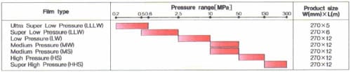
Figure 2.1: Applicable pressure ranges for Fuji Pre-scale Films [2]
The films are available in two possible formats. One format is based on two sheets. The other is based on a single sheet. The film types MS (Medium pressure) and HS (High pressure) are single sheet layered types. The other Fuji film types are two sheet layered types.
Single sheet film< /p>
The single sheet film type consists of a polyester base, with a coated color developing layer on it. The micro encapsulated color forming material is layered on top of the film as can be seen in figure 2.2a.
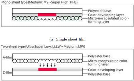
Figure 2.2: Both Pre-scale formats from Fuji Prescale instruction sheet
Two sheets film
The double layered Pre-scale film is composed of an A film (made of a polyester base) which is coated with microcapsules filled with color forming material. The C film (also made of a polyester base) is coated with a color developing material. To use these films, make sure the coated surfaces are facing each other. Otherwise there will be no footprint (see figure 2.2b).
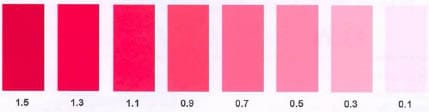
Figure 2.3: Magenta sample table
2.2 Momentary pressure measurement
With the Fuji Pre-scale films an Extended pressure measurement and a Momentary pressure measurement can be done. When using the extended pressure method, the applied pressure should increase gradually to its maximum in five seconds, before the pressure is kept constant for about two minutes. In a momentary pressure measurement the applied pressure should be gradually increased to the highest magnitude in five seconds, and it should be maintained here for another five seconds. After these five seconds at the highest level, the pressure has to be gradually released. This type of measurement could also be used for impact measurements.
Because a momentary pressure measurement simulates a tyre/road contact the most realistic, all measurements in this project are momentary pressure measurements. To convert the obtained color densities from the Fuji Pre-scale films to a pressure, the Momentary Pressure Chart has to be used (see appendix A).
The momentary pressure chart consists of several curves which depend on the temperature and the relative humidity. The proper curve has to be selected before the color densities can be converted to a pressure. To select the proper curve, one needs to measure the temperature and relative humidity first. With these values known, the proper area can be selected from the reference chart (see figure 2.4). The selected area corresponds to the proper pressure chart curve.
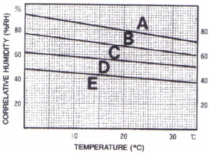
Figure 2.4: Reference chart for type LLLW from Fuji Prescale reference sheet
Chapter 3
Calculations with MATLAB
3.1 Implementing in MATLAB
To make calculations in MATLAB with the obtained footprints, the Fuji Pre-scale films have to be digitalized. A MATLAB file will be written to calculate the contact surface and pressure distribution. With use of a flatbed scanner the films can easily be digitalized. The films must be scanned on True Color with a known resolution. This chapter describes how the digitalized footprint can be implemented in MATLAB.
Mean Pixel Values
The MATLAB function imread is used to calculate the contact surface and the pressure distribution. This function is available in the standard MATLAB toolboxes, although it is recommended to install the image processing toolbox. The function reads all pixel values from a picture file and returns the data in an array. If the file contains a grayscale image the array is a two dimensional array of size M by N, where M is the number of pixels in horizontal direction and N is the number of pixels in vertical direction. When a color picture file is imported, the array is three dimensional. Each layer in this array represents one of the RGB colors.
In this project, the obtained magenta footprints are converted to grayscale, resulting in a M by N matrix. The rows of the matrix contain the number of pixels in horizontal direction and the columns contain the number of pixels in vertical direction. Each individual pixel has a mean pixel value, which corresponds to a certain color and thus to a pressure. To convert a mean pixel value to a pressure, the curves of the both Momentary Pressure Charts (for type LLW and type LLLW) have to be implemented in the MATLAB file. In a momentary pressure chart the pressure is a function of the color density (this density corresponds to a color from the magenta sample table (figure 2.3) [2]). Therefore the densities from this magenta sample table have to be converted to mean pixel values first.
This is done with use of MATLAB. The magenta sample table is converted to grayscale and a histogram in which every peak correspond to a certain color density is created (see figure 3.2). The total number of pixels is plotted against all possible grayscale colors and corresponding mean pixel values. A pixel value of 0 means absolutely black and a value of 255 means absolutely white. Every value in between is a unique gray color.
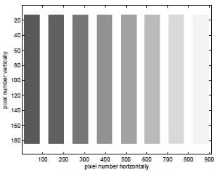
Figure 3.1: Magenta sample table converted to grayscale
The mean pixel values corresponding to the densities from the magenta sample table can easily be found. Table 3.1 gives these values. When fitting a 3rd order polynomial through these points, one can determine for every color density the corresponding pixel value (see appendix B).
Table 3.1: Density with according mean pixel value
Summarized: Every scanned pixel from the Fuji Pre-scale film has its own pixel value. This pixel value corresponds to a color density and using the momentary pressure charts, the corresponding pressure can be calculated.
3.2 The MATLAB file
This section describes the working principle of the written MATLAB file, also called m-file. The m-file is a function file and named contact1.m. The m-file is added in appendix D.
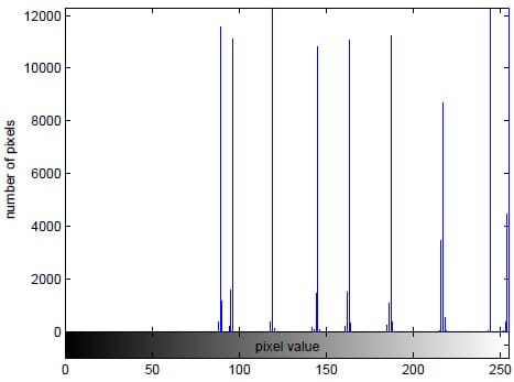
Figure 3.2: Histogram of the sample table
Input arguments
Before running the function file, the following input has to be given in:
contact1(’picturename.ext’,dpi,humidity,temperature,’type’,inflationpressure,force).
In the input argument ’picturename.ext’ the filename with its extension (for example: .jpg, .bmp, .png etc.) has to be given in. The filename and extension have to be placed between quotation marks. Dpi stands for ’Dots per inch’ and represents the resolution of the scanned Fuji Pre-scale films. The third and fourth input arguments are the relative humidity and the temperature of the lab during the measurements. For the input argument ’type’ the used film type has to be given. Two types can be chosen and must also been placed between quotation marks. The first type is the LLLW film type, the second type is the LLW film type. Finally, the inflation pressure of the car tyre (in bars) and the vertical applied force have to be filled in.
Contact surface
The m-file starts with reading the picture from the file and displays it. This colored picture will be converted to grayscale with 256 grayscale colors. The number of pixels are counted as a function of all possible pixel values and a histogram of the picture will be plotted. The sum of all the pixels is the total number of pixels of the picture.
Because the used Fuji Pre-scale films have color densities from 0.1 to 1.5, corresponding to mean pixel values of 244 to 89, the lowest pixel value that will occur will be 89 and the highest occurring pixel value (that corresponds to a color) will be 245. Therefore pixel value 245 will be the highest value in the color range
. Pixel value 30 will be the minimum of the color range. This color range is chosen because otherwise there will be no difference any more between a grayscale color and black or white. The sum of the pixels with pixel values in the color range is the total number of color pixels.
With the total number of color pixels known MATLAB calculates the percentage color of the picture. The total surface of the picture and also the surface of the colored pixels can be calculated using the dpi. Because a colored pixel means contact (the color forming material has reacted with the color developing material), the surface of the colored pixels equals the contact surface.
Mean pressure and vertical force
To convert the pixel values to pressures, the momentary pressure charts have to be used. These charts are implemented in the m-file for both types of films, using a 3rd order polynomial fit. Also the curves of the reference charts for both types are implemented, to choose the proper pressure chart curve. MATLAB selects the proper pressure chart curve, using the temperature and humidity.
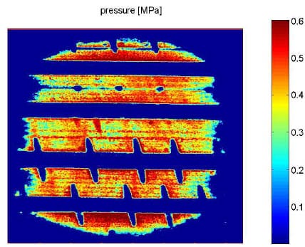
Figure 3.3: Pressure distribution on a contact surface
The next step is to determine the pressure of every individual pixel to visualize the pressure distribution (figure 3.3). When all the pressures are add up and divided by the sum of the total color pixels, one gets the mean pressure. Multiplying the mean pressure and the contact surface results in the applied vertical force.
3.3 Comparing both m-files
P.W. Backx [1] already wrote a MATLAB file (named contact.m) to make calculations with the Fuji films. This m-file does not calculate for every pixel value the according density, but only for ranges of pixel values together. For example: a pixel has a pixel value of 141. Because the pixel value 141 is close to the pixel value 145, the m-file takes the pixel value 145 for this pixel. A pixel value of 145 corresponds to a color density of 0.9 as can be seen in table 3.1. In the same way pixels with pixel value 247 (outside the color range) could become 244.
For the current project a new m-file is written. This m-file calculates for every pixel value the according color density (see appendix D). The working principle of the m-file is described in section 3.2.
In this section both m-files are being compared. This will be done by checking the calculated contact surface with known contact surfaces and by checking the calculated percentage color of a file with a known percentage color.
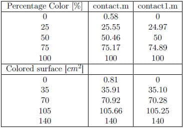
Table 3.2: Comparison of the results of both m-files
Both m-files have calculated the percentage color of a file and the surface of the colored pixels. The percentages color and the surfaces of the colored pixels are known and depict in the left column of table 3.2. As can be seen from the table the file contact.m is not very precise. Although there is no color at all, the m-file gives a color percentage and a surface. The other calculated surfaces are also too high in comparison to the m-file written for this project.
A last comparison is made using the measured footprint from [1]. To make an estimation of the contact surface and color percentage of the footprint, a grid is being drawn using Adobe Photoshop 7.0 and the colored squares with dimensions of 5 x 5 mm are being count (see figure 3.4).
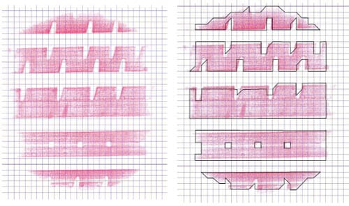
Figure 3.4: Contact surface estimation
There are 360 out of 986 squares colored. This corresponds to a color percentage of:
360/986 · 100 = 36.51%
and the contact surface follows from:
360 · 0.5 · 0.5 = 90 cm2.
When running both m-files the results from table 3.3 are obtained. The results of the file contact.m are again not as precise as the m-file contact1.m. Therefore the file contact1.m will be used for the continuation of this project.
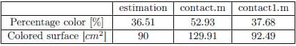
Table 3.3: Results of both m-files
Chapter 4
Experiments
4.1 Select film type
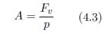
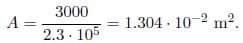
Before starting a measurement using the pressure sensitive Fuji Pre-scale Films, the most suitable film type has to be chosen first. As mentioned before there are different applicable pressure ranges for these films, varying from type LLLW (Ultra Super Low Pressure) to type HS (High pressure). To select the most suitable film type, a simple calculation can be made. Assuming the nominal weight of a loaded car is 1600 kilograms and the vertical loads acting on the car are evenly distributed on all four wheels, each wheel has to deal with a vertical force Fv of
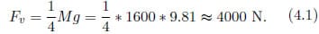
With the vertical force per wheel known and an assumption for the contact surface between the car tyre and the road, one can calculate the mean contact pressure p using the following equation:
Taking a contact width of 0.15 meter and a contact length of 0.12 meter, the mean contact pressure follows from equation 3.2:
This pressure is a mean value, so higher and lower peak values occur. When taking the profile of a car tyre into account also, it is obvious that the mean contact pressure increases (because of the decrease in contact surface). Therefore the most suitable film type has to have an applicable pressure range beginning with at most 0.2 MPa. The only film type satisfying this pressure range is the LLLW type.
However, when high peak values in pressure are expected, for example in a contact pressure measurement between a tyre and a gravel road or rough asphalt, the LLLW pressure range is too small and may saturate too quickly. Using the LLW film type, with an applicable range of 0.5 MPa to 2.5 MPa, may solve this problem. Unfortunately there are two disadvantages in comparison with the LLLW film type: the LLW film type is less accurate and a pressure below 0.5 MPa cannot be measured.
4.2 Measurement setup
To measure the pressure distribution of a contact surface, use is being made of pressure sensitive Fuji Pre-scale Films. Under the influence of an applied external force, these films will color magenta (described in more detail in chapter 2). Using MATLAB, these color densities can be converted into pressures.
All the measurements took place in the Automotive Engineering Science lab of the faculty Mechanical Engineering. Here they have a tyre measuring machine, the so-called flat plank tyre tester (see figure 4.1). On this machine, all forces acting on the tyre can be applied under realistic tyre/road boundary conditions and also low velocities or camber can be simulated and measured. Since we are only interested in the pressure distribution on a contact surface, only an applied vertical force and no camber or velocity is needed. For every contact pressure measurement, a new film type has to be fixed on the flat plank and a vertical force has to be applied with the car tyre. With an LVDT (Linear Variable Differential Transformer) sensor attached to the tyre tester, one can measure the vertical displacement of the car tyre also. Appendix C gives a short description of how an LVDT sensor works.
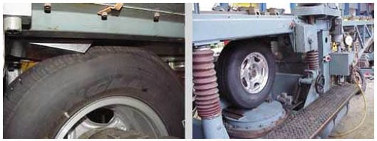
Figure 4.1: Flat plank tyr
e tester [3]
4.3 Measurements
4.3.1 Different measurement configurations
For this Bachelor Final Project, eight different measurements were done. The tyre used for all these measurements is a Continental SportContact2 225/50 R17 98Y (see figure 4.2). Two measurements were done on asphalt using the LLWfilm type, with an inflation pressure of 2.3 bars and a vertical force of 4000 Newton. The other six measurements were done on the flat plank with different forces and inflation pressures, using the LLLW film type (see table 4.1). The situation with an inflation pressure of 2.3 bars and a vertical force of 4000 Newton was measured by P.W Backx [1]. Because the results are still available, there is no need to measure this situation again.
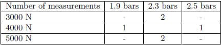
Table 4.1: Different measurement configurations
4.3.2 Laboratorium circumstances
To convert the color densities from the Fuji Pre-scale Films to a correct pressure, the proper conversion curve has to be selected. For this, one needs to measure the temperature and the relative humidity of the laboratorium. The best operating temperature to use the Fuji Pre-scale Films is between 25 °C and 30 °C. The best operating humidity lies between 30 % and 80 %.
In [1] the temperature of the laboratorium was 20 °C with a relative humidity of 53 %. In the present project, before starting a measurement on asphalt, a temperature of 22.1 °C and a relative humidity of 33 % were measured. The next four measurements on the flat plank were measured in a relative humidity of 45 % with a temperature of 23.4 °C. The circumstances of the lab during the last two measurements on the flat plank (the first measurement with 3000 Newton, the second with 5000 Newton and both with an inflation pressure of 2.3 bars) were 65 % relative humidity and 22.5 °C in temperature.

Figure 4.2: Footprint of the Continental SportContact2
4.3.3 Load profiles
As mentioned before, all measurements are momentary pressure measurements. In these measurements the vertical load has to be applied, kept constant and released in fifteen seconds. The vertical load as a function of time can be visualized in a load profile. For the asphalt measurements the both load profiles are displayed in figure 4.3.
The vertical force is applied by hand, so it is very difficult to keep the force for exactly five seconds constant. Due to relaxation effects of the tyre, a maximum peak in the load profiles occur.
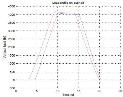
Figure 4.3: Load profiles for both asphalt measurements
4.4 Tyre/road contact surfaces
In this section the obtained footprints measured with the Fuji Pre-scale Films are displayed. The conversion of these footprints to pressure profiles and other calculations using MATLAB (for example determining the contact area, the mean pressure and vertical stiffness) are discussed in the next chapter.
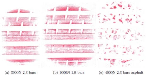
Figure 4.4: Three different footprints obtained from measurements
The real size footprints are scanned and scaled to the dimensions of the figure above. One can see the differences between the contact surfaces. All obtained footprints are scanned with 300 dots per inch. Figure 4.4c shows the high peak pressures occurring when a tyre and an asphalt road are making contact. Because the LLW film type is used for this measurement, only the pressures higher than 0.5 MPa are visible. As can be seen, these high pressure values only occur on the asphalt grains. Between these grains, lower pressures exists, however the values are below 0.5 MPa and so the LLW Fuji Pre-scale Film does not color magenta there. It can be expected that this effect will influence the mean contact pressure and the pressure distribution calculations.
One can make an apparent contact surface estimation, using a designer program such as Corel DESIGNER 12. To do so, an ellipse must be drawn with the same dimensions as the scanned footprint. Using the designer program, the surface of the ellipse can easily be found. With an apparent surface estimation the grooves are not taken into account.
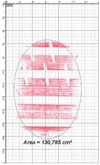
Figure 4.5: Contact surface estimation
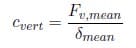
To compare this estimated surface with the theoretical expectation, equation 4.2 has to be rewritten into:
Taking an inflation pressure of 2.3 bars and an applied vertical force of 3000 N, the theoretical surface follows from equation 4.3:
This method is a rough estimation for the apparent contact surface. Depending on the shape and exactitude of the ellips.
Chapter 5
Results
5.1 Theoretical Expectations
There exist many equations to predict the contact length of a contact surface. The contact length is a function of the tyre radius, vertical load, vertical stiffness and inflation pressure of the tyre. Before predicting the length of a contact surface, first the vertical tyre stiffness and the tyre deflection have to be determined.
An equation to determine the theoretical vertical tyre stiffness is given in [4] and for the situation with no tyre velocity this equation simplifies to:
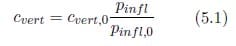
where pinfl,0 is the nominal tyre pressure (pinfl,0 = 2 · 105 [N/m2]) and cvert,0 the reference vertical tyre stiffness at pinfl = pinfl,0. When the tyre stiffness is known, the tyre deflection can easily be calculated using equation 5.2.
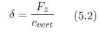
With this deflection, half of the contact length can be estimated using a relation provided by Besselink [5]:
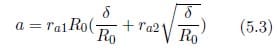
where R0 is the tyre radius and ra1 = 0.35 and ra2 = 2.25.
A m-file is written to predict the deflections, tyre stiffness and the contact lengths using the equations presented above.
Before calculating the vertical tyre stiffness, the reference vertical tyre stiffness cvert,0 has to be known. Cvert,0 is the vertical tyre stiffness with an inflation pressure of two bars. For the present project no measurements with inflation pressures of two bars were done. However the vertical tyre stiffness of the measurements with inflation pressures of 1.9 bars and 2.3 bars are known. Therefore a lineair interpolation between these values of stiffness is done to determine cvert,0.
The predicted values following from equations 5.1, 5.2 and 5.3 are summarized in table 5.1. These values will be checked by the results of the measurements. The measured vertical tyre stiffness and the deflection of the tyre will be calculated using the m-file totalstiffness.m (see appendix E). The contact length of the obtained footprints
will be measured.
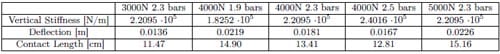
Table 5.1: Prediction of vertical stiffness, deflection and contact length
Contact lengths
The measured contact lengths CL and contact widths CW of the obtained footprints are depicted in table 5.2.
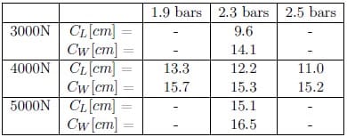
Table 5.2: Measured contact lengths and contact widths
As can be seen the calculated contact length for the situation with 5000N applied force and an inflation pressure of 2.3 bars is a good estimation for the measured contact length. The estimations for the contact lengths of the situations with 4000N applied force and inflation pressures of 1.9 bars and 2.5 bars, are approximately two centimeters too high. For the situation with an inflation pressure of 2.3 bars and an applied vertical force of 3000N, the estimation also differs approximately two centimeters. The estimation of situation [1] differs approximately one centimeter.
Because the contact length predictions of the m-file are thus not very precise, the m-file will be modified. This will be done using table 5.2 and correction factors. The contact widths will also be added to the m-file. For the contact widths usually a percentage of the tyre section width will be taken. The tyre used for all measurements has a section width of 225 mm. A rough estimation for the contact width can be made when taking 70 % of the section width for an applied vertical force of 5000N. For an applied vertical force of 4000N 65 % of the section width has to be taken. Sixty percent of the section width is taken for an applied vertical force of 3000N.
When modifying the m-file with these descriptions the results of table 5.3 are obtained. The m-file is attached to appendix F.
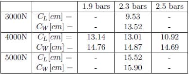
Table 5.3: Calculated contact lengths and contact widths
The theoretical determined vertical tyre stiffness and tyre deflections of table 5.1 will be compared to calculated values from the measurements in the next section.
5.2 Vertical tyre stiffness
To determine the vertical stiffness of the tyre, the deflection of the tyre and applied force have to be measured. The applied force as function of time can be plotted in a load profile. The force is kept constant at a specific level for five seconds. For these five seconds the applied force is at its maximum, and a mean applied vertical force can be calculated for this interval.
The displacement of the car tyre is measured using an lvdt sensor. The measured displacement in the output file is the displacement of the lvdt sensor (and thus of the car tyre) but not the deflection of the car tyre.
This will be explained using figure 5.1. As can be seen in the displacement graph, the black curve (corresponding to the displacement of the output file and thus to the displacement of the car tyre) gives a displacement before a force is applied. After 7.5 seconds the black curve decreases as the applied force is released. However the curve does not stop with a displacement of zero millimeters, but with a negative value of displacement. Explanation: before applying a force to the tyre, the tyre does not touch the road. When starting a measurement (t = 0 seconds) the tyre is displaced towards the road, resulting in a displacement of the pushrod of the lvdt sensor. The tyre still does not touch the road, so there is no applied force yet. When the tyre hits the road, a force on the tyre is applied which will gradually be increased to its maximum. If the maximum value is reached, the force is kept constant and the tyre will not displace. After five seconds the force has to be gradually released and the tyre will come off the road again. When the distance between the road surface and the car tyre is larger afterwards than it was before the measurement, the lvdt sensor gives a negative displacement.
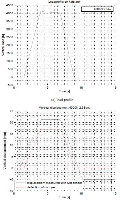
Figure 5.1: Load profile and tyre displacement
To calculate the deflection of the car tyre the measured displacement graph has to be corrected. This is been done using a m-file named totalstiffness.m (see appendix E). First has to be determined the displacement of the lvdt sensor when the force is applied. Because when the force is applied, the car tyre starts to deflect. This value of displacement is being subtracted from all measured displacement points as function of time to get the deflection graph of the car tyre. Also the negative displacements have to be converted to a zero displacement. In this way there will be a positive tyre deflection when the force is applied and there will be no tyre deflection if the tyre does not touch the road. The deflection of the car tyre as function of time is plotted in the displacement graph.
In the same interval as the force is kept constant the deflection will be constant. Therefore a mean deflection is being calculated for this interval. When dividing the mean applied vertical force by the mean tyre deflection, one can calculate the vertical tyre stiffness.
The mean tyre deflections are depicted in table 5.4. The deflection of the tyre with an inflation pressure of 2.3 bars and an applied vertical force of 4000N from [1] is unknown because P.W. Backx did not measure deflections. The estimated deflections of table 5.1 look very precise for the first measurements. When the first two situations are measured again, the values from the second measurements are obtained. These deflections are a bit larger than the deflections of the first measurements.
This can be explained because the pushrod of the lvdt sensor used for the measurements is very distorted. Because of this the sensor has to be bend straight before starting a measurement. For the second measurements the lvdt sensor could be not bend straight enough and therefore a larger deflection is measured.
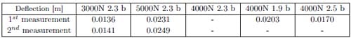
Table 5.4: Calculated mean deflections of car tyre
The m-file totalstiffness.m calculates the mean vertical tyre stiffness for every inflation pressure (because the inflation pressure influences the stiffness) and also for the asphalt measurements a mean vertical tyre stiffness is being calculated. This because the influence of asphalt on the tyre stiffness is unknown. The results are displayed in table 5.5.
The asphalt influences the tyre stiffness a little as can be seen in table 5.5. However this is not representative. When not taken the vertical tyre stiffness on asphalt into account, the estimated values of table 5.1 are a good approximation for the first measurements. Because the deflections of the measurements done for the second time are higher than those of the first time, the calculated vertical stiffness will be lower.
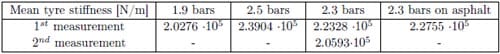
Table 5.5: Calculated mean vertical tyre stiffness
5.3 Contact surface and mean pressure
The theoretical apparent contact surface can be calculated using equation 4.3. The apparent contact surface can also be estimated using the ellipse method. In table 5.6 the error between the theoretical apparent surface and the estimated apparent surface is shown.
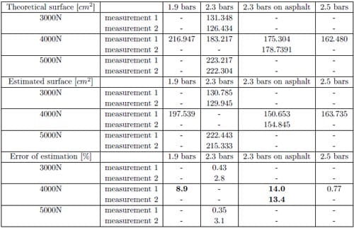
Table 5.6: Theoretical surface and surface estimation
The error of the estimated surface depends on the exactitude of the ellipse and of the shape of the contact surface. The contact s
urface obtained with an applied vertical force of 4000N and an inflation pressure of 1.9 bars has a rectangular shape (see figure 5.4) and can thus not be estimated very precise using an elliptical shape. It is also very difficult to determine the shape of the footprints obtained from asphalt measurements (see figure 5.5), therefore this method is not very precise to estimate the contact surface of an asphalt measurement.
With use of the calculated surface from the m-file Ac and the theoretical surface At, the void ratio can be determined. This can be done using the following equation:
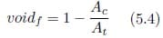
The theoretical mean pressure on a contact surface is higher than the inflation pressure of the tyre, due to the grooves of the tyre. It is obvious that a higher void ratio corresponds to a higher mean contact pressure. To calculate this theoretical mean contact pressure, use is being made of an equation from Michelin [6]:
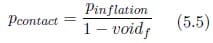
The results are depicted in tables 5.7 and 5.8. The most extreme values are displayed in bold type. These values will be discussed.
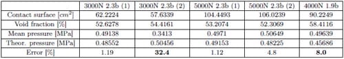
Table 5.7: Comparison of measurement results (part one)
3000N 2.3 bars
The results of the first measurement with an inflation pressure of 2.3 bars and an applied vertical force of 3000N were very precise. An error of only 1.19 % occurred. Therefore the Fuji pressure sensitive films look very applicable for this configuration. To confirm this, the measurement is done twice. When the error of the second measurement is very small again, the applicability of the Fuji films for the current configuration looks perfect. The used reference curve for the first measurement was curve D. During the second measurement, the circumstances of the lab were 65% of humidity and the temperature of the lab was 22.5 °C. With these circumstances, reference graph C has to be used.
Unfortunately during the second measurement several pixels did not color magenta. The reason for this can be found in the way the double layered films were attached to the flat plank. The double layered sheets may not taped tight enough to the flat plank and therefore several pixels did not color magenta because they were fold double or did not make any contact to the flat plank. This is also the reason why the calculated contact surface of the second measurement is lower than it was the first measurement. A smaller calculated surface leads to a higher void ratio, which results in the increase of the theoretical mean pressure. As can be seen, the calculated mean pressure of the second measurement is much lower than the calculated mean pressure of the first measurement. This results in an error of more than 30 percent. Therefore no conclusions from this measurement can be drawn about the applicability of the Fuji films with an applied vertical force of 3000N.
See figure 5.2 for the differences between both footprints and figure 5.7 for the pressure distribution of both measurements.
Table 5.8: Comparison of measurement results (part two)
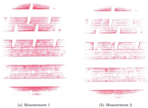
Figure 5.2: Measurement with 3000N applied force and inflation pressure of 2.3 bars
5000N 2.3 bars
The error of the second measurement with an applied vertical force of 5000N and an inflation pressure of 2.3 bars is 4.8 %. This error is higher than the error of the first measurement. When looking at both footprints, the colored pixels of the second measurement are looking darker colored magenta than the colored pixels of the first measurement (the pixels of the second measurement seem to have a higher color intensity). This can be checked by plotting the histograms of both measurements. As follows from these histograms, the colored pixels of measurement two are darker colored magenta than the colored pixels of measurement one indeed. When the same vertical force is applied with the same inflation pressure of the tyre in measurement two, another conversion curve has to be used. This because the pixels of the second measurement are darker colored. Darker colored pixels mean higher contact pressures. The higher occurring pressures are corrected using another conversion curve (otherwise the pressures of the second measurement would become higher than the pressures of the first measurement and this is not expected). When the used conversion curve is not very accurate, it could explain the error of the second measurement.
The calculated contact surface of the second measurement is larger than the first calculated contact surface. This can be explained because the dimensions of the Fuji film used for the first measurement were too small and therefore the total footprint did not fit on the Fuji film (as can be seen in figure 5.3). Because of this and the lower void fraction, the theoretical contact pressure is lower than it was the first time.
The obtained footprints and calculated pressure distributions look very similar (see figure 5.3 and figure 5.6). Therefore no huge measurement faults are expected and because the first measurement was very precise, conversion curve C may be inaccurate. Before concluding this, another measurement has to be done in the same circumstances of the lab.
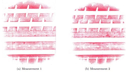
Figure 5.3: Measurement with 5000N applied force and inflation pressure of 2.3 bars
4000N 1.9 bars
The calculated surface of the measurement with an applied vertical force of 4000N and 1.9 bars is too small. This because several pixels did not color magenta (see the white circles in figure 5.4). A smaller contact surface results in a higher void ratio. The theoretical mean pressure will therefore increase. Every colored pixel corresponds to a pressure. When all these pressure values are summed up and divided by the total number of colored pixels, the mean pressure is calculated. The mean contact pressure should be equal to the theoretical mean contact pressure. For this measurement the error is 8.0 %. Because the calculated surface is too small in comparison to the measurement with an applied vertical force of 4000N and an inflation pressure of 2.3 bars (this because a lower inflation pressure results in a lower tyre stiffness and therefore in a higher contact surface), the theoretical mean contact pressure will also be too high. This may be a reason for the error of 8.0 %. Another reason for this error may be a measurement fault. Another measurement with the same configurations has to be done to investigate this. When the error of the second measurement is also about eight percent, the Fuji pressure sensitive films may not be very applicable for this configuration.
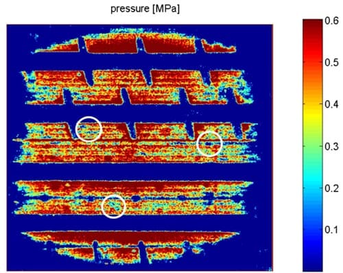
Figure 5.4: Pressure distribution 4000N 1.9 bars
On every footprint, one can see horizontal lines where pixels are colored darker magenta and lines where pixels are colored lighter magenta. These lines are for every footprint the same (see for example the pressure distributions). This could be the structure of the flat plank.
Asphalt measurements
For the asphalt measurements both errors are high. This was expected because these measurements were done with use of the LLW film type. With this type of film only the pressures higher than 0.5 MPa are visible. These pressures only occur on the asphalt
grains. Between these grains, lower pressures exists, however the values are below 0.5 MPa and so the LLW Fuji Pre-scale Film does not color magenta there (see figure 5.5). Therefore the m-file only calculates the contact surface of the asphalt grains.
The pressure range of the LLW film type starts with 0.5 MPa, therefore the obtained color densities correspond to pressures higher than 0.5 MPa.
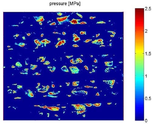
Figure 5.5: Pressure distribution 4000N 2.3 bars on asphalt
The calculated mean pressure on the asphalt grains is 1.014 MPa for the first measurement. For the second measurement this value equals 1.089 MPa. Because only the contact surface of the grains is calculated and not the contact surface between these grains, a correct void ratio cannot be calculated. Therefore equation 5.5 is not applicable.
To measure the total contact surface (the grain contact surface as well as the contact surface between these grains) and the total mean pressure occurring on a tyre/road contact, a Fuji Pre-scale Film with a larger range is needed. For example a range from 0.2 MPa to 2.5 Mpa. Unfortunately Fuji films with these ranges does not exist.
One may solve this problem measuring the same situation with both film types. The LLLW film type can be used to calculate the total contact surface and the occurring pressures between the grains. The LLW film type can be used to determine the maximum occurring pressures. Combining both results gives the mean pressure and pressure distribution. To combine both film types and results, the m-file has to be rewritten.
Calculating the vertical applied force
To calculate the applied force, the calculated contact surface and mean pressure have to be multiplied. Because the calculated mean pressure consists of an error, the calculated applied force will have the same error.
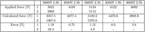
Table 5.9: Calculated applied vertical force with error
The mean applied vertical force can be obtained from the m-file totalstiffness.m. Table 5.9 gives the results.
Pressure distributions
A pressure distribution can be drawn using the pressure value of every individual pixel. The pressure distributions of the measurements done twice are displayed on the next two pages. The differences between both measurements are more obvious using pressure distributions.
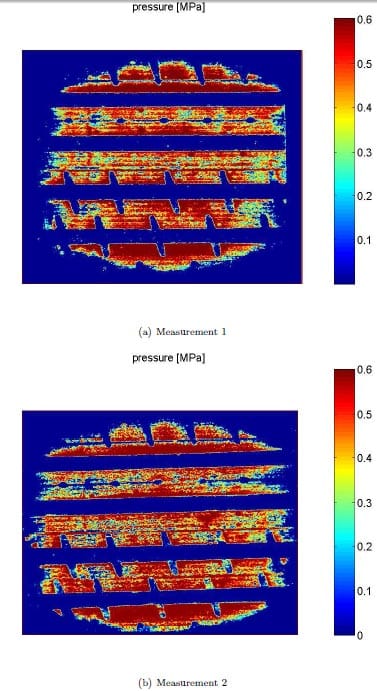
Figure 5.6: Pressure distribution 5000N 2.3 bars
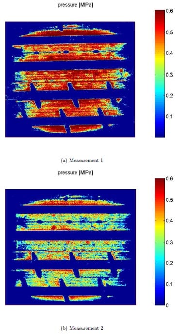
Figure 5.7: Pressure distribution 3000N 2.3 bars
Chapter 6
Conclusions and recommendations
6.1 Conclusions
The results of the measurements on the flat plank, using the Fuji Pre-scale films with an applied vertical force of 4000N and an inflation pressure of 2.3 bars or 2.5 bars, were satisfying. Therefore the Fuji Pre-scale films seem to be a good method to measure the mean pressure and pressure distribution with these configurations. It must be mentioned these results are obtained using conversion curve D. When using the pressure sensitive films on asphalt, the applicable pressure ranges of the Fuji Pre-scale films are not satisfying. Using film type LLW results in colored pixels corresponding to pressures higher than 0.5 MPa, which will only occur on the asphalt grains. The LLW film type cannot measure the pressures between these grains. The film type LLLW can, but may saturate too quickly. Combining both film types may be a solution.
The results of the first measurement using an applied vertical force of 5000N and an inflation pressure of 2.3 bars were very precise. An error of only 1.12 % occurred. The conversion curve used is curve D. For the second measurement the conversion curve C had to be used because of the circumstances of the lab. The error of this measurement was 4.8%. Because another conversion curve is used, it is very difficult to draw a conclusion. The Fuji Pre-scale films seem to be very applicable on measurements using an applied vertical force of 5000N when conversion curve D is used. Another measurement in area C has to be done before it is clear whether this curve is inaccurate or the 4.8% error is due to measurement faults.
The results of the first measurement with an applied vertical force of 3000N looked very good. To confirm the good applicability of the pressure sensitive films using this configuration, more measurements are needed because during the second measurement a measurement fault occurred.
No conclusions from the measurements can be drawn about the applicability of the Fuji Prescale films as an alternative cost-effective way to measure contact pressures. Before doing this more measurements with the same conditions and circumstances are needed.
6.2 Recommendations
There are a couple of recommendations for further investigations of the Fuji films. Because the results of the measurement with an applied force of 5000N and an inflation pressure of 2.3 bars were very good, using conversion curve D, also measurements in other regions can be done to check the accuracy of all conversion curves. The second measurement with an applied vertical force of 3000N failed because of measurement faults, so other measurements using conversion curve D have to be done to determine the applicability of the Fuji Pre-scale films with this value of applied force. Measurements with other configurations (for example: 3000N applied force and 1.9 bars inflation pressure or 5000N applied force and 2.5 bars inflation pressure) can be done to investigate the applicability of the films with these configurations.
To investigate the applicability of these films on asphalt, measurements with both types of film have to be done and the results have to be combined. Recommended are measurements on asphalt with a smaller grain size.
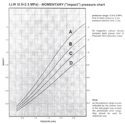
Figure A.1: Momentary Pressure Chart LLW [2]
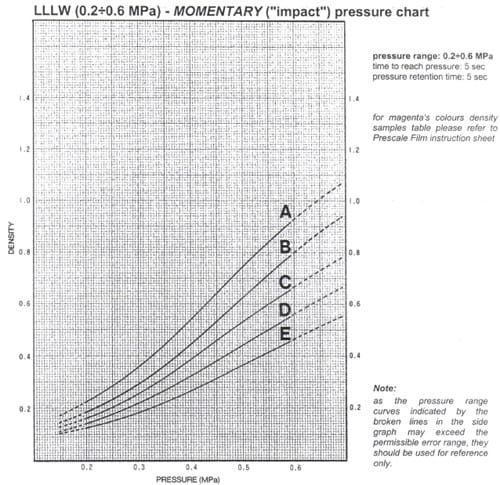
Figure A.2: Momentary Pressure Chart LLLW [2]
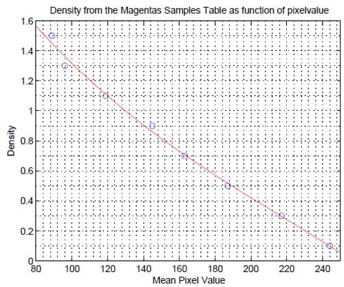
Figure B.1: 3rd order polynomial fit through mean pixel values
The LVDT sensor
LVDT stands for Linear Variable Differential Transformer. An LVDT sensor is a displacement measuring instrument. The displacement calculations of this sensor are not based on strains. The LVDT sensor is based upon two secondary coils, symmetrically wound on to one primary coil. When moving the push rod, the high permeability core displaces. This movement determines the voltage induced from the primary coil to each secondary coil. The output voltage is a lineair function of displacement. For example: when moving the rod three centimeters to the right, the output voltage is +5 V. Moving the rod three centimeters to the left, the output voltage is -5 V.
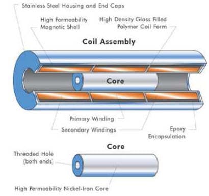
Figure C.1: The primary and two secondary coils of an LVDT sensor [7]
M-file: Contact1.m
function [ ] = contact1(’picturename.ext’,dpi,humidity,temperature,’type’,inflationpressure,force).
%This function calculates the mean contactpressure in MPa and %the contactarea in cm^2, measured with pressure sensitive %Fuji Prescale Film.
%Define th
e picturename as a string (’picturename.ext’, … ), %Dpi (dots per inch), humidity and temperature must be given as %integers. The input ’type’ requires to select which type of Fuji Prescale %film is used (i.e. ’LLLW’ or ’LLW’). The inflation pressure has to be in %bars and the vertical applied force in Newton.
close all clc warning off all %%%%%%%%%%%%%%%%%%%%%%%%%%%%%%%%%%%%%%%%%% % Reading the image % %%%%%%%%%%%%%%%%%%%%%%%%%%%%%%%%%%%%%%%%%%
pic = imread(picturename); %read picture from file image(pic); %display 8bit RGB picture xlabel(’Pixel number horizontally’); ylabel(’Pixel number vertically’); title(’Loaded picture in color’)
%%%%%%%%%%%%%%%%%%%%%%%%%%%%%%%%%%%%%%%%%%%%%%%%%%%%%%%%%%%%%%%%%%%%%%%%%%% %Calculate the monochrome luminance by combining the RGB values according % %to the NTSC standard, which applies coefficients related to the eye’s % %sensitivity to RGB colors. % %%%%%%%%%%%%%%%%%%%%%%%%%%%%%%%%%%%%%%%%%%%%%%%%%%%%%%%%%%%%%%%%%%%%%%%%%%% graypic = .2989*pic(:,:,1)+.5870*pic(:,:,2)+.1140*pic(:,:,3);
%%%%%%%%%%%%%%%%%%%%%%%%%%%%%%%%%%%%%%%%% % Plot pictures % %%%%%%%%%%%%%%%%%%%%%%%%%%%%%%%%%%%%%%%%%
%Grayscale figure;
colormap(gray(256)) %use grayscale colormap with 256 colors
image(graypic);
xlabel(’Pixel number horizontally’);
ylabel(’Pixel number vertically’);
title(’Loaded picture in grayscale’)
%Histogram
figure;
imhist(graypic)
[COUNTS, X] = imhist(graypic); %Count number of pixels as a function of
[COUNTS, X]; %the mean pixelvalue.
TotalPixels = sum(COUNTS);
xlabel(’Mean pixel value’);
ylabel(’Number of pixels’);
title(’Histogram’)
%Plot Counts and pixelvalue
figure;
plot(X,COUNTS) %Only the pixelvalues who
axis([30 245 0 20000]); %correspondent to a color are plotted.
xlabel(’Mean pixel value’); %(pixels with values between 30 and 245)
ylabel(’Number of pixels’); %Because color = contact!
title(’Number of pixels against Mean pixel value (in colorrange)’)
grid;
%%%%%%%%%%%%%%%%%%%%%%%%%%%%%%%%%%%%%%%%%%%%%%%%%%%%%%%%%%%%%%%%%%%%%%% % Calculating the Total Color Pixels % %%%%%%%%%%%%%%%%%%%%%%%%%%%%%%%%%%%%%%%%%%%%%%%%%%%%%%%%%%%%%%%%%%%%%%%
pic2 = imread(picturename); h = ones(5,5)/25;
pic2 = imfilter(pic2,h);
graypic = .2989*pic2(:,:,1)+.5870*pic2(:,:,2)+.1140*pic2(:,:,3);
try
if type == ’LLW’
TotalColorPixels = sum([COUNTS(30:255)]);
end
catch
if type == ’LLLW’
TotalColorPixels = sum([COUNTS(30:245)]);
end
end picture = double(graypic);
x = [89:1:255];
k = 0;
for i = 1:length(picture(:,1))
for j = 1:length(picture(1,:))
if picture(i,j) > 244 | picture(i,j) < 89
k = k +1;
end
end
end
%disp([’number of pixels outside colorrange = ’,num2str(k)]);
%%%%%%%%%%%%%%%%%%%%%%%%%%%%%%%%%%%%%%%%%%%%%%%%%%%%%%%%%%%%%%%%%%%%%%%%%% % Calculating pressure as function of mean pixel value for type = LLW % %%%%%%%%%%%%%%%%%%%%%%%%%%%%%%%%%%%%%%%%%%%%%%%%%%%%%%%%%%%%%%%%%%%%%%%%%%
LLWpixelA = [238 231 217 202 187 175 163 154 145 132 119 108 96];
LLWpressureA = [0.2875 0.4 0.625 0.825 1.025 1.2 1.375 1.55 1.7125
1.8625 2.075 2.275 2.5];
LLWpA = polyfit(LLWpixelA,LLWpressureA,3);
LLWfA = polyval(LLWpA,x);
LLWpixelB = [238 231 217 202 187 175 163 154 145 132 119];
LLWpressureB = [0.3625 0.4875 0.7375 0.9875 1.2 1.4125 1.625 1.825 2.025 2.225 2.475];
LLWpB = polyfit(LLWpixelB,LLWpressureB,3);
LLWfB = polyval(LLWpB,x);
LLWpixelC = [244 231 224 217 202 187 175 163 154 145 132];
LLWpressureC = [0.3 0.5875 0.725 0.875 1.1375 1.3875 1.6375 1.8625 2.1 2.35 2.5];
LLWpC = polyfit(LLWpixelC,LLWpressureC,3);
LLWfC = polyval(LLWpC,x);
LLWpixelD = [244 238 231 224 217 202 187 175 163 154];
LLWpressureD = [0.3625 0.525 0.7125 0.8875 1.05 1.35 1.65 1.925 2.2 2.4875];
LLWpD = polyfit(LLWpixelD,LLWpressureD,3);
LLWfD = polyval(LLWpD,x);
try
if type == ’LLW’
filmtype = ’LLW’;
C1 = humidity + (29/35)*temperature – 95;
C2 = humidity + (37/35)*temperature – 84;
C3 = humidity + (24/35)*temperature – 58;
if C1 > 0usedcurve = ’A’;
for i = 1:length(picture(:,1))
for j = 1:length(picture(1,:))
if picture(i,j) < 96 %Pixels with lower pixelvalues
picture(i,j) = 96; %than 96 correspond to pressures
elseif picture(i,j) > 224 %higher than 2.5 Mpa and the
picture(i,j) = 0; %film saturates. The LLW film type
end %pressure range starts with 0.5 Mpa,
%and lower pressures cannot
%be measured.
for m = 89:255
if picture(i,j) == m
pressure(i,j) = polyval(LLWpA,picture(i,j));
end
end
end
end
elseif C2 > 0
usedcurve = ’B’;
for i = 1:length(picture(:,1))
for j = 1:length(picture(1,:))
if picture(i,j) < 119
picture(i,j) = 119;
elseif picture(i,j) > 230
picture(i,j) = 0;
end
for m = 89:255
if picture(i,j) == m
pressure(i,j) = polyval(LLWpB,picture(i,j));
end
end
end
end
elseif C3 > 0
usedcurve = ’C’;
for i = 1:length(picture(:,1))
for j = 1:length(picture(1,:))
if picture(i,j) < 132
picture(i,j) = 132;
elseif picture(i,j) > 235
picture(i,j) = 0;
end
for m = 89:255
if picture(i,j) == m
pressure(i,j) = polyval(LLWpC,picture(i,j));
end
end
end
end
else
usedcurve = ’D’;
for i = 1:length(picture(:,1))
for j = 1:length(picture(1,:))
if picture(i,j) < 154
picture(i,j) = 154;
elseif picture(i,j) > 239
picture(i,j) = 0;
end
for m = 89:255
if picture(i,j) == m
pressure(i,j) = polyval(LLWpD,picture(i,j));
end
end
end
end
end
end
catch
if type ==’LLLW’
filmtype = ’LLLW’;
%%%%%%%%%%%%%%%%%%%%%%%%%%%%%%%%%%%%%%%%%%%%%%%%%%%%%%%%%%%%%%%%%%%%%%%%%% % Calculating pressure as function of mean pixel value for type = LLLW % %%%%%%%%%%%%%%%%%%%%%%%%%%%%%%%%%%%%%%%%%%%%%%%%%%%%%%%%%%%%%%%%%%%%%%%%%%
C1 = humidity + (22/35)*temperature – 92;
C2 = humidity + (16/35)*temperature – 76;
C3 = humidity + (12/35)*temperature – 62;
C4 = humidity + (10/35)*temperature – 48;
LLLWpixelA = [231 224 217 210 202 187 175 163 154 145];
LLLWpressureA = [0.17 0.22 0.26 0.295 0.325 0.38 0.43 0.4775 0.53 0.585];
LLLWpA = polyfit(LLLWpixelA,LLLWpressureA,3);
LLLWfA = polyval(LLLWpA,x);
LLLWpixelB = [238 231 224 217 210 202 187 175 163 154];
LLLWpressureB = [0.15 0.215 0.265 0.305 0.34 0.375 0.43 0.485 0.5425 0.6];
LLLWpB = polyfit(LLLWpixelB,LLLWpressureB,3);
LLLWfB = polyval(LLLWpB,x);
LLLWpixelC = [238 231 224 217 210 202 187 175 169];
LLLWpressureC = [0.185 0.25 0.295 0.3375 0.375 0.41 0.4775 0.55 0.5875];
LLLWpC = polyfit(LLLWpixelC,LLLWpressureC,3);
LLLWfC = polyval(LLLWpC,x);
LLLWpixelD = [238 231 224 217 210 202 195 187 175];
LLLWpressureD = [0.215 0.28 0.3325 0.38 0.4225 0.465 0.505 0.5475 0.6];
LLLWpD = polyfit(LLLWpixelD,LLLWpressureD,3);
LLLWfD = polyval(LLLWpD,x);
LLLWpixelE = [238 231 224 217 210 202 195 187];
LLLWpressureE = [0.25 0.325 0.385 0.435 0.485 0.535 0.59 0.6];
LLLWpE = polyfit(LLLWpixelE,LLLWpressureE,3);
LLLWfE = polyval(LLLWpE,x);
if C1 > 0
usedcurve = ’A’;
for i = 1:length(picture(:,1))
for j = 1:length(picture(1,:))
if picture(i,j) < 145 %Pixels with lower pixelvalues
picture(i,j) = 145; %than 145 correspond to
end %pressures higher than 0.6 Mpa
%and the film saturates.
for m = 89:245
if picture(i,j) == m
pressure(i,j) = polyval(LLLWpA,picture(i,j));
end
end
end
end
elseif C2 > 0
usedcurve = ’B’;
for i = 1:length(picture(:,1))
for j = 1:length(picture(1,:))
if picture(i,j) < 154
picture(i,j) = 154;
end
for m = 89:245
if picture(i,j) == m
pressure(i,j) = polyval(LLLWpB,picture(i,j));
end
end
end
end
elseif C3 > 0
u
sedcurve = ’C’;
for i = 1:length(picture(:,1))
for j = 1:length(picture(1,:))
if picture(i,j) < 169
picture(i,j) = 169;
end
for m = 89:245
if picture(i,j) == m
pressure(i,j) = polyval(LLLWpC,picture(i,j));
end
end
end
end
elseif C4 > 0
usedcurve = ’D’;
for i = 1:length(picture(:,1))
for j = 1:length(picture(1,:))
if picture(i,j) < 175
picture(i,j) = 175;
end
for m = 89:245
if picture(i,j) == m
pressure(i,j) = polyval(LLLWpD,picture(i,j));
end
end
end
end
else
usedcurve = ’E’;
for i = 1:length(picture(:,1))
for j = 1:length(picture(1,:))
if picture(i,j) < 187
picture(i,j) = 187;
end
for m = 89:245
if picture(i,j) == m
pressure(i,j) = polyval(LLLWpE,picture(i,j));
end
end
end
end
end
end
end
%%%%%%%%%%%%%%%%%%%%%%%%%%%%%%%%% % Plot pressure distribution %%%%%%%%%%%%%%%%%%%%%%%%%%%%%%%%%
mesh(pressure);
colormap jet
colorbar
view(2)
axis off
xlabel(’number of pixels horizontally’)
ylabel(’number of pixels vertically’)
title(’pressure [MPa]’)
%%%%%%%%%%%%%%%%%%%%%%%%%%%%%%%%%%%%%%%%%%%%%%%%%%%%%%%%%%%%%%%%%%%%%%%%% % Calculating mean contact pressure and Vertical Force % %%%%%%%%%%%%%%%%%%%%%%%%%%%%%%%%%%%%%%%%%%%%%%%%%%%%%%%%%%%%%%%%%%%%%%%%%
totalpressure = 0;
n=0;
for i = 1:length(pressure(:,1))
for j = 1:length(pressure(1,:))
if pressure(i,j) > 0
totalpressure = totalpressure + pressure(i,j);
n = n + 1;
end
end
end
PercentageColor = TotalColorPixels / TotalPixels * 100;
ContactArea = TotalColorPixels * (0.0254/dpi)^2 *10^4; % [cm^2]
Meanpressure = totalpressure/TotalColorPixels;
Fz = (Meanpressure*10^6) * (ContactArea*10^-4);
At = force/(inflation_pressure*10^5)*10^4;
Voidfraction = (1 – (ContactArea/At))*100;
Pc = inflation_pressure/(1 – (Voidfraction/100))*10^-1;
%%%%%%%%%%%%%%%%%%%%%%%%%%%%%%%%%%%%%%%%%%%%%%%%%%%%%%%%%%%%%%%%%%%%%%%% % Display input variables and output % %%%%%%%%%%%%%%%%%%%%%%%%%%%%%%%%%%%%%%%%%%%%%%%%%%%%%%%%%%%%%%%%%%%%%%%%
disp([’humidity = ’,num2str(humidity)])
disp([’temperature = ’,num2str(temperature)])
disp([’used filmtype = ’,filmtype])
disp([’used reference chart = ’,usedcurve])
disp([’dpi = ’,num2str(dpi)])
disp([’inflation pressure = ’,num2str(inflation_pressure)])
disp([’applied vertical force = ’,num2str(force)])
disp([’ ’])
disp([’Color = ’, num2str(PercentageColor), ’ %’])
disp([’Contactarea = ’, num2str(ContactArea), ’ [cm^2]’])
disp([’Meanpressure = ’,num2str(Meanpressure), ’ [Mpa]’])
disp([’Vertical Force = ’,num2str(Fz), ’ [N]’])
disp([’Theoretical Contactarea = ’, num2str(At), ’ [cm^2]’])
disp([’Voidfraction tyre = ’, num2str(Voidfraction), ’ %’])
disp([’Theoretical Contactarea pressure = ’,num2str(Pc), ’ [Mpa]’])
M-file: Vertical Stiffness
E.0.1 Total vertical stiffness
%%%%%%%%%%%%%%%%%%%%%%%%%%%%%%%%%%%
% The file totalstiffness.m calculates the mean vertical tyre stiffness.
% For every new inflation pressure, a new mean vertical stiffness is
% determined.
% This m-file loads the eight other m-files and uses the calculated
% answers.
close all
clc
clear all
%%%%%%%%%%%%%%%%%%%%%%%%%
%loading the other m-files
p4000N19b;
p3000N23b;
p4000N25b;
p5000N23b;
p4000N23b_asphalt1;
p4000N23b_asphalt2;
pL5000N23b;
pL3000N23b;
%%%%%%%%%%%%%%%%%%%%%%%
%calculating the mean vertical tyre stiffness
Kv_gem_asphalt = (Kv4000N23b_asphalt1 + Kv4000N23b_asphalt2)/2
Kv_gem_19bars = Kv4000N19b
Kv_gem_23bars_measurement1 = (Kv5000N23b_1 + Kv3000N23b_1 )/2
Kv_gem_23bars_measurement2 = (Kv5000N23b_2 + Kv3000N23b_2 )/2
Kv_gem_25bars = Kv4000N25b
Kv_gem_asphalt =
2.2755e+005
Kv_gem_19bars =
2.0276e+005
Kv_gem_23bars_measurement1 =
2.2328e+005
Kv_gem_23bars_measurement2 =
2.0593e+005
Kv_gem_25bars =
2.3904e+005
E.0.2 Tyre stiffness per measurement
%%%%%%%%%%%%%%%%%%%%%%%%%%%%%%%%%%%%% % Load .txt file
load ’pL4000p19.txt’
Fz = pL4000p19(:,3);
disp = pL4000p19(:,6);
a = length(Fz);
b = a/2;
t = [0.01:0.01:(a/100)];
%%%%%%%%%%%%%%%%%%%%%%%%%%%%%%%%%%%%%
% Plot vertical Force
figure
hold on
plot(t,pL4000p19(:,3), ’k’)
xlabel(’Time [s]’)
ylabel(’Vertical load [N]’)
title(’Loadprofile on flatplank’)
legend(’4000N 1.9bar’)
grid minor
%%%%%%%%%%%%%%%%%%%%%%%%%%%%%%%%%%%%%
% Plot measured displacement of lvdt sensor
figure
hold on
plot(t,pL4000p19(:,6), ’k’)
%%%%%%%%%%%%%%%%%%%%%%%%%%%%%%%%%%%%%%
% Calculate time when force is applied
k=0;
for m = 1:b
if Fz(m,1) <= 0
k = k+1;
end
end
j = (k+1);
t0 = j/100;
%%%%%%%%%%%%%%%%%%%%%%%%%%%%%%%%%%%%
% Determine displacement of sensor when force is applied
zerodisp = disp(j,1);
c = pL4000p19(:,6) – zerodisp ; %When force is applied, tyre deflection
%starts with 0 mm.
%%%%%%%%%%%%%%%%%%%%%%%%%%%%%%%%%%%%
% Plot deflection tyre
for e=1:a
if c(e,1) < 0
c(e,1) = 0;
end
end
plot(t,c, ’r’)
xlabel(’Time [s]’)
ylabel(’Vertical displacement [mm]’)
title(’Vertical displacement 4000N 1.9Bars’)
legend(’displacement measured with lvdt sensor’,’deflection of car tyre’)
grid minor
%%%%%%%%%%%%%%%%%%%%%%%%%%%%%%%%%%%%
% Calculate vertical stiffness
Fzmean = sum([Fz(500:815)])/316;
dispmean = sum(([c(500:815)])/316)/1000;
Kv4000N19b = Fzmean/dispmean;
M-file: Contact length estimation
function []=contactlength1(Sectionwidth,AR,Drim,pressure,loadpertyre) close all
%%%%%%%%%%%%%%%%%%%%%%%%%%%%%%%%%%%%%
% This function calculates the contact length and vertical stiffness of a
% car tyre, based on emperical formulas.
% The section width (mm), aspect ratio, diameter of the rim (inches),
% inflations pressure in bars) and the load per tyre (N)
% have to be filled in.
%%%%%%%%%%%%%%%%%%%%%%%%%%%%%%%%%%%%%
%Calculating the contact length
Fv =loadpertyre;
%Calculating vertical stiffness of the car tyre(Kt)%
Diarim = Drim * .0254; %Converting inches to meters
b = Sectionwidth * 10^-3;
cvert0 = 1.9213*10^5; %[N/m]
pressure0 = 2; %[bars]
Kt = cvert0 * (pressure/pressure0)
%Calculating the contact length Cl and contact width Cw
deflection = Fv/Kt
Height_tyre = b*AR/100;
Radius_tyre = (Height_tyre*2 + Diarim)/2;
a = 0.35*Radius_tyre*((deflection/Radius_tyre) + 2.25*sqrt(deflection/Radius_tyre));
if pressure == 2.3
Cl = 2*a + ((1*10^-5*Fv) -0.05)
else
Cl = 2*a – 0.02
end
Cw = (Fv*5*10^-5 + 0.45)*b
M-file: Reference graphs
%%%%%%%%%%%%%%%%%%%%%%%%%%%%%%%%%%%%%%%%%%%%%%%%%%%%%%%%%%%%%%%%%%%%%%% % Creating Fuji Prescale temperature-humidity graph for LLW filmtype % %%%%%%%%%%%%%%%%%%%%%%%%%%%%%%%%%%%%%%%%%%%%%%%%%%%%%%%%%%%%%%%%%%%%%%%
close all
clc
T = 0:1:35; %Define temperature (T) range
h1LLW = – (29/35)*T + 95;
h2LLW = – (37/35)*T + 84;
h3LLW = – (24/35)*T + 58;
figure;
plot(T,h1LLW, ’r’)
axis([0 35 0 100]);
xlabel(’Temperature (Degree Celsius)’)
ylabel(’Correlative Humidity (%RH)’)
title(’Graph of temperature and humidity for type = LLW’)
hold on
plot(T,h2LLW, ’g’)
plot(T,h3LLW, ’b’)
grid;
%%%%%%%%%%%%%%%%%%%%%%%%%%%%%%%%%%%%%%%%%%%%%%%%%%%%%%%%%%%%%%%%%%%%%%%% % Creating Fuji Prescale temperature-humidity graph for LLLW filmtype % %%%%%%%%%%%%%%%%%%%%%%%%%%%%%%%%%%%%%%%%%%%%%%%%%%%%%%%%%%%%%%%%%%%%%%%%
h1LLLW = -(22/35)*T + 92;
h2LLLW = -(16/35)*T + 76;
h3LLLW = -(12/35)*T + 62;
h4LLL
W = -(10/35)*T + 48;
figure;
plot(T,h1LLLW, ’r’)
axis([0 35 0 100]);
xlabel(’Temperature (Degree Celsius)’)
ylabel(’Correlative Humidity (%RH)’)
title(’Graph of temperature and humidity for type = LLLW’)
hold on
plot(T,h2LLLW, ’g’)
plot(T,h3LLLW, ’b’)
plot(T,h4LLLW, ’m’)
grid;
%%%%%%%%%%%%%%%%%%%%%%%%%%%%%%%%%%%%%%%%%%%%%%%%%%%%%%%%%%%%%%%%%%%%%%%% % Plot density with according mean pixel value % %%%%%%%%%%%%%%%%%%%%%%%%%%%%%%%%%%%%%%%%%%%%%%%%%%%%%%%%%%%%%%%%%%%%%%%%
Density = [.1 .3 .5 .7 .9 1.1 1.3 1.5]’;
MeanPixelValue = [244 217 187 163 145 119 96 89]’;
x = [80:1:255];
p = polyfit(MeanPixelValue,Density,3);
f = polyval(p,x);
density = f’;
[density, x’];
figure;
plot(MeanPixelValue,Density,’o’)
axis([80 250 0 1.6])
hold on
plot(x,f,’r’)
grid minor;
xlabel(’Mean Pixel Value’)
ylabel(’Density’)
title(’Density from the Magentas Samples Table as function of pixelvalue’)
References
- P.W. Backx, Tyre/road contact measurement using pressure sensitive films, Eindhoven University of Technology, DCT 2007.026 (2007)
- FujiFilm, Fuji Prescale Pressure Measuring Film instruction sheets, Fuji Film Imaging and Information
- https://www.automotive.tno.nl
- J. de Hoogh, Implementing inflation pressure and velocity effects into the Magic Formula tyre model, Eindhoven University of Technology, Master Thesis DCT-2005.46 (2005)
- I.J.M. Besselink, Vehicle Dynamics lecture notes 2003, Eindhoven University of Technology, (2003)
- Michelin, CD-ROM volume 3 ’Le pneu/The tyre/Der reifen’
- https://www.macrosensors.com