
Article
Related Links
By: Alberto Makino, William R. Hamburgen, John S. Fitch
Abstract
The elastic properties of gum rubber and fluoroelastomers were studied by a variety of numerical and experimental methods. Results were applied to the design of flat pressure pads for microelectronic applications. The goal was to develop an understanding sufficient that designers could quickly develop acceptable fluoroelastomer pressure pads without further detailed studies. The effort centered on optimizing the performance of a 14 mm square by 0.8 mm thick pad under a fixed normal force. The primary optimization criterion was minimization of the maximum normal contact stresses applied by the pad to a rigid surface.
Judicious perforation of flat pads greatly reduced adverse contact stress gradients. The preferred design used four 1.2 mm holes symmetrically arrayed in a 4 mm square grid centered on the pad. Compared to an unperforated pad, this arrangement yielded a 28% reduction in maximum contact stresses.
1 Introduction
Flat sheets of rubber are frequently used to transfer a load from one planar surface to another. Such pads serve to reduce local pressure nonuniformities due to point defects (bumps and voids), as well as large scale distortions (warp, bow, waviness). But owing to the incompressibility of rubber, the pressure applied by a pad is not truly uniform, rather it tends to be highest at the center of the pad, decreasing toward the edges. In some microelectronic applications, such as when the pad contacts the active surface of a silicon microcircuit (die), this pressure nonuniformity is of tremendous importance. Rubber pad use in packaging can be temporary or permanent. An example of temporary application occurs when a pad is used to load the adhesive joint during high pressure die attach as shown in Fig.1. The ball pivot keeps the spring force centered on the die, while the rubber pad distributes the force preventing excessive or spatially varying normal contact stresses which may cause die cracking or a nonuniform adhesive thickness distribution [1]. An example of permanent rubber pad application is depicted in Fig.2, where the pad is used in a package to press the die against a heatsink in order to form a pressure contact joint. A similar approach was used for a recent Siemens mainframe computer [2, 3]. In this case, contact stress gradients can lead to corresponding temperature gradients. Figure 2 also shows the importance of understanding pad deformation; if the edges of the pad bulge excessively, bondwire damage may occur. And in both cases, shear tractions applied to the active surface of the die may damage it.
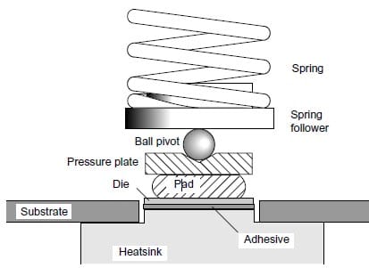
Figure 1: High pressure adhesive die attach process.
Our laboratory had previously designed such pads by empirical methods, but we wanted to move toward higher pressures for both die attach and pressure contact heat transfer applications. We were concerned about the effects of contact pressure nonuniformity, and decided to embark on the current study.
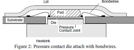
Figure 2: Pressure contact die attach with bondwires.
The force distribution could bemodified by using a pad with a 3-Dsurface profile rather than a flat surface. To reduce costs and lead times, we chose instead to investigate the limitations of shapes stamped from flat stock with low cost punches and steel-rule dies. The Siemens mainframe is also reported to have used perforated pads [4].
We chose two elastomers for our investigation. The first was pure gum rubber, since it is one of the materials whose properties have been most widely reported in the open literature. The second was VitonTM [Du Pont], the fluoroelastomer we had already selected for our end use applications. Viton has excellent chemical resistance and tolerates high temperatures 1 . And while it is much more expensive than conventional compounds, it is a fraction of the cost of fully fluorinated elastomers such as KalrezTM [Du Pont] and ChemrazTM [Green, Tweed, & Co.]. Viton is also readily available in sheet form in both commercial and MIL-SPEC grades; this proved to be an important distinction. Viton is the commercial name of copolymers of vinylidene fluoride. Several types are available: Viton “A” is a dipolymer of vinylidene fluoride and hexafluoropropylene, Viton “B” and “F” are terpolymers of vinylidene fluoride and combinations of hexafluoropropylene and tetrafluoroethylene [5]. The main difference is their chemical resistance to aggressive substances. The elongation at break is rather low (about 200%) and these compounds are generally stiffer than other rubber-like materials [6].
The goal of our research was to develop a sufficient understanding of the behavior of small Viton pads, so that designers could quickly develop acceptable pressure pad designs without further detailed studies. Both numerical and experimental methods were used. Our work centered on optimizing the behavior a 14 mm square by 0.8 mm thick pad under a fixed normal force. Our primary optimization criteria was minimization of the maximum normal contact stresses applied by the pad surface.
2 Rubber Elasticity
2.1 Finite Elasticity
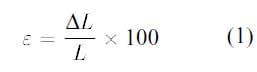
Rubber and rubber-like materials have the unique capability to withstand large deformations and still be able to fully recover their original dimensions. These materials owe their unusual properties to theirmolecular structure, which consists of long hydrocarbon chains (oftenwithCl or Fl substitutions) with a tangled shape and freely rotating links. The hydrocarbon molecules are interlocked in such a way that they form a three dimensional network able to sustain large deformations as chains straighten (Treloar [7] p.12.) Natural and syntehtic rubbers and their derivatives can achieve strains as high as 500%-1000%. In this case “strain” is defined as the percentage change in original length L.
Calculation 1
By contrast, most other engineering materials are only able to recover their initial dimensions for strains of at most a few tenths of a percent in uniaxial extension. Within those limits, both rubber and other solids behave elastically, which implies not only the recovery from any imposed deformations but also independence of stresses on previous deformation history.
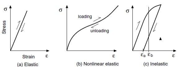
Figure 3: Types of stress-strain responses
Engineering materials such as crystalline metals are classified as linear elast
ic solids whereas rubber-likematerials are considered nonlinear elastic solids. The difference is the type of stress strain behavior as shown in Fig.3. These curves represent the stress-strain response to unixial loading. Figure 3(a) depicts the constant slope response associated with a linear isotropic Hookean material, a class to which most metals belong. Figure 3(b) depicts a behavior typical of rubber-like solids, in which stresses cannot be described as a linear function of strains. In both cases however, the curves during loading and unloading follow the same path; the stress is a unique function of the strain or deformation. Figure 3(c) depicts a third case where the stresses are not a single-valued function of the strains. Stresses during loading and unloading follow different paths. For a given strain, such as εb, there are two possible stress values depending on previous loading history. Also, note that upon unloading to zero stress, the material has acquired a permanent deformation εa. This is called inelastic behavior, and is typical of materials when the elastic limit is exceeded.
Deformations inmetals loadedwithin the elastic limits aremuch less than unity and therefore their behavior can usually be adequately characterized with either a strength of materials approach or its more refined counterpart, the infinitesimal theory of elasticity. Rubber-like materials can exhibit strains that are several orders of magnitude higher, and the same approach cannot be used. The more general finite elasticity theory is needed. All measures, such as strains and stresses, defined for linear isotropic elastic solids have to be recast in the context of a finite deformation theory. It is noted that the infinitesimal theory constitutes a limiting case of the finite deformation theory. Only the fundamental concepts of finite elasticity will be presented here; the interested reader is referred to the many excellent treatises on continuum mechanics and nonlinear elasticity such as Malvern [8], Green and Adkins [9], and Green and Zerna [10].
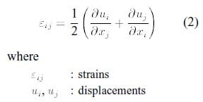
One of the main differences between the infinitesimal and finite deformation theories is the location at which the stress and strain measures are defined. When deformations are large, the initial and final locations of a particular point such as P in Fig.30 (Appendix A, page 39)may be widely separated. In such cases, motions, strains, and stresses could be defined in two different ways, by referencing them to the initial undeformed configuration or to the current deformed configuration. These are the Lagrangian and Eulerian descriptions [8]. When deformations are small compared to unity, as with metals, this distinction becomes unnecessary and all stress and strain measures collapse into the definitions of the infinitesimal theory. The strain tensor, defined in the infinitesimal theory in terms of displacement gradients as is replaced in finite elasticity theory by either the Lagrangian or Eulerian finite strain tensor, EAB or eij(see Appendix A, page 40 and ref.[8]).
Calculation 2
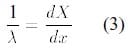
Although it is possible to analyze rubber-like materials using finite strains, it is customary to instead use a stretch ratio, λ, defined in the deformed configuration as the ratio of the original and current relative lengths.
Calculation 3
The only differences are the values at zero deformation, where the stretch ratio is λ=1 but the Lagrangian and Eulerian strains are E = e = 0. A stretch ratio of λ=2 in a given direction indicates that the final dimension is twice the original one. The use of stretch ratios in finite elasticity is a matter of convenience due to the magnitude of the deformations. By contrast, using stretch ratios in the infinitesimal theory would be cumbersome at best. For example, an object with an original length of 1 mm and a final length of 1.001 mm, is much easier to describe using engineering strains (ε=0.1%).
Stress measures in finite elasticity theory center around the Cauchy or true stresses which are defined in the deformed configuration2.
2.2 Stresses and Constitutive Equations
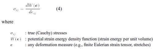
In most engineering design problems, the load acting on an object is known, or can be assumed to fall within in a certain range. Based on this, the analyst seeks to determine the corresponding effects in the interior of a solid, i.e., investigate stresses and their distribution. Stresses cannot be measured directly and must instead be related to measurable quantities such as strains or stretch ratios through the use of constitutive equations which describe the relationship between stresses and stretch ratios or strains. The independence of stresses on previous deformation history and the reversibility of imposed deformations in elastic materials allows us to prove that constitutive relations for both linear and nonlinear elastic solids can be derived from a strain energy potential function. This argument is very similar to the path independent work done on a particle in a potential field where the forces can be derived from a differentiable potential function [11]. By analogy, if stresses take the place of forces, a differentiable potential function must exist3 that it is a function only of the deformations. In such cases stresses can be expressed as
Calculation 4
Any material for which such a potential strain energy function exists is called a Green-elastic or hyperelastic material [8]. In the strictest terms, both linear and nonlinear elastic materials are hyperelastic. In practice however, the term hyperelastic is generally applied only to rubber-like materials. From the mathematical standpoint, there are two ways to apply Eq.4 to obtain a constitutive relation. One is to assume small strains, take a series expansion and consider only the linear terms. This leads to the familiar Hooke’s law for linear elastic solids. The other is to assume finite strains and construct a suitable strain energy function. The success of any analytical or numerical effort in hyperelastic solids depends closely on the ability of the chosen strain energy function to reproduce the actual material behavior.
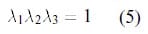
In spite of their compliant appearance, most rubbers are incompressible or nearly incompressible solids. This makes them capable of withstanding large hydrostatic tractions without any change in volume and implies that deformations alone cannot describe stress states in the interior of such materials. For example, imagine a rubber ball deep in the ocean. It is subjected to homogeneous external tractions p = pgh(p: water density, g: acceleration of gravity, h: depth), yet due to its imcompressibility, it has the same dimensions as at sea level. This incompressibilty condition can be expressed as a function of the stretch ratios along three orthogonal directions,
Calculation 5
Our focus here will be on homogenous deformations, those in which the deformation gradient Fi,A does not depend on the original configuration X(see Appendix A, page 40). Such deformations can be completely characterized with only three stretch ratios along orthogonal directions. The hydrostatic state of the ball in the ocean example is one case. Another is a sample subjected to biaxial extension along two orthogonal axes. Since the unit vectors associated with the original and deformed configurations (Nand n) do not change orientation in a homogeneous deformation, th
ere is only one stretch measure (see Appendix A, page 41).
In the general case of an isotropic hyperelastic solid, the strain energy density function W must be a symmetrical function of the stretch ratios λ1, λ2, and λ3 (see Rivlin [12] and Treloar [7].) It follows that Wcan be defined in terms of the three invariants defined as,
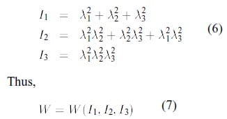
Calculation 6 and 7
The choice of W can be arbitrary as long as it does not violate any of the principles of continuum mechanics (for example, it must predict zero stress at zero deformation). A suitable general form is a power series of the invariants I1, I2, I3.
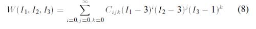
Calculation 8
where Cijk = material constants.
This function is zero at zero deformation as long as C000 = 0. Also note that by Eq.6, I1 = I2 = 3 and I3 = 1 for λ1 = λ2 = λ3 = 1, and the correct zero stress is predicted by Eq.4.
When the incompressibility condition is introduced, I3 = 1 for any stress state, and the terms affected by it drop from Eq 8 giving
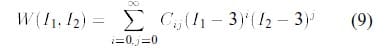
Calculation 9
Again, C00 = 0 in order to have zero stresses at zero deformation. Generally the first few terms in the series dominate, and we can consider W be given by the two-term approximation which includes only the linear terms in I1 and I2 (i=1; j=0 and i=0; j=1),
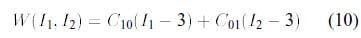
Calculation 10
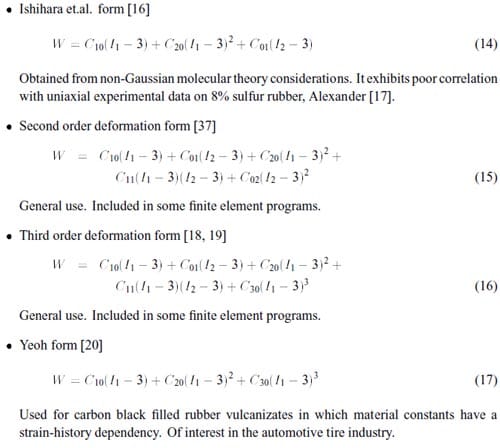
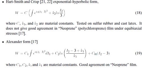
This is perhaps the form most widely used in rubber elasticity and is known as the Mooney- Rivlin strain energy function, first proposed by Mooney in 1940 [13, 12]. The Mooney-Rivlin form has been found to reproduce the behavior of most natural and synthetic rubbers for moderate deformations (λ = 4). For higher stretch ratios it is less successful, and over the years, a number of other forms for the strain energy function have been proposed in response to the need to characterize a variety of rubber-like materials. Some of these are higher order approximations of Eq.9 and others have been formulated along rather different lines, among them:
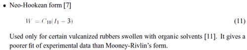
Calculation 11
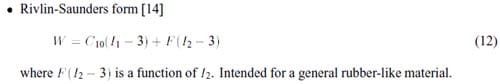
Calculation 12
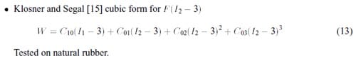
Calculation 13

The choice of a strain energy function depends heavily on the material and the stretch ratios to which it will be subjected. For relatively small stretch ratios, say λ<2, a linear approximation such as Mooney-Rivlin’s is usually quite adequate, but for high stretch ratio ranges, a higher order approximation may be needed.
Once a strain energy function is chosen, one must still determine the material constants Cij, μi, etc., and the expression for the stresses. Considering stretch ratios as deformationmeasures, the stresses are expressed using Eq.4,
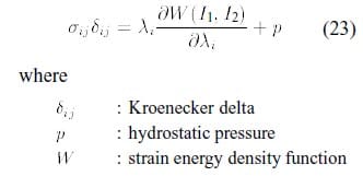
The additional term, p, can be considered a Lagrange multiplier needed to comply with the incompressibility condition and accounts for any hydrostatic tractions. For example, a uniaxial loading along the first axis can be described by the stretch ratios
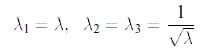
(since λ1 is imposed, λ2 and λ3 are considered to be equal and obtained from the imcompressibility condition, λ1λ2λ3 =1). If a Mooney-Rivlin material and zero hydrostatic tractions are assumed, then the stresses from Eq.23 are

2.3 Application to Pad Design
The objective of our investigation was to optimize the contact stress distribution in flat Viton pads under a specified normal load. If contact at the pad faces were frictionless, the problem would reduce to one of equibiaxial loading. The pad would expand uniformly, maintaining its original shape, and the contact stresses would be uniform. But in real assemblies the contact is not frictionless. As a bounding case, one can assume perfect friction or adhesion at the pad faces. Since rubber-like materials experience nearly isochoric (volume preserving) deformations, any kinematic constraints that tend to confine thewhole or part of thematerial cause stress gradients. When friction is introduced, Fig.4, the central part of the pad experiences a stiffening response to the lateral confinement. By contrast, portions near the edges are still able to move relatively freely. This gives rise to substantial radial stress gradients. Placing a hole or perforation in the zone where confinement is expected allows the surrounding material to flow toward the hole’s free edge, relieving contact stresses in the vicinity. Our investigation was intended to explore the combined effects of hole placement and size on the contact stress distribution and to reduce its peak value.
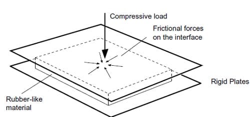
Figure 4: Effect of a finite friction coefficient on material confinement.
In spite of their deceptively simple appearance, the closed form calculation of stresses from the analytical expressions presented so far can be made only in a limited number of cases with simple geometries, boundary conditions, and homogeneous deformations. Experimental methods can be used instead if the time and expense are justified. For example, the contact stress distribution in compressed rubber cylinders has been successfully analyzed by such a method [24]. However, in the vast majority of design cases where direct solutions are not possible the widespread availability of numerical methods such as nonlinear finite element analysis has reduced the need for experimentalmethods. Commercial codes that include several hyperelastic constitutive models are routinely used in the tire and automotive industries [19]. We chose the same approach to evaluate our pad designs. But first, we needed to determine the material constants for Viton.
3 Material Characterization
In order to use the constitutive models offered by finite element codes, it is necessary to provide values for the various material constants (Cij) defined in the previous section. Unfortunately, there is a wide variation in the properties of synthetic rubbers owing to the large number of compounding variants. The few material constants that have been published in the open literature are for commonly used products such as natural and vulcanized rubbers and pure gum rubber [11]. In practice, it is necessary to characterize each material of interest. This is done by recordi
ng the stress-stretch ratio response for simple loading cases and performing a least squares fit of the data to an appropriate constitutive relationship. Since different loading modes have slightly different stress-stretch ratio responses, the test loading must be representative of the problem under consideration. It would be incorrect to use material constants obtained, say from an extension test, in a finite element model loaded under pure shear. If the primary loading mode is unknown, then several tests under different loading types are needed and the constitutive model fitted to all experimental points.4
The most common homogeneous deformation tests are: Uniaxial extension, Equibiaxial extension, Pure shear.
However, the primary loading mode of interest in the design of pressure pads is uniaxial compression. Curiously enough, the superposition principle can be used to show that uniaxial compression of awide sheet (e.g. a pressure pad) is equivalent to uniformequibiaxial extension. To visualize this, consider the sheet in Fig.5(a),which is subjected to equibiaxial tractions δ, and also subjected to a hydrostatic stress state -δ. By the superposition principle, the hydrostatic tractions at the edge of the sheet exactly cancel the tractions imposed by the equibiaxial extension. But the faces of the sheet are still subjected to the hydrostatic tractions. The net result is a sheet loaded in uniaxial compression. Hence, we choose an equibiaxial test as the primary means for obtaining material constants for Viton pressure pads.
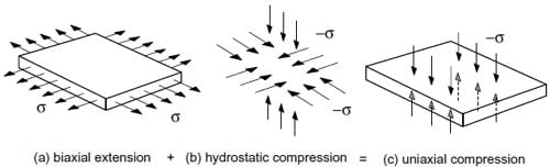
Figure 5: Equivalency of uniform biaxial extension and uniaxial compression
There are several ways to obtain biaxial extension. One of them involves stretching a sheet of rubber in two orthogonal directions. However, there are a number of problems with this method: the difficulty ofmaintaining a constant 1:1 load ratio on the two loading directions and the clampingmethod. Clampingmust usually be donewith strings in order to avoid nonuniform transmission of the imposed load to the sheet. The load ratio problem can be solved by using dead weights, springs, or a feedback control system with active loading devices. An additional problem is to maintain the load alignment with respect to the deforming sheet (remember the large deformations that rubber can attain). A detailed description of the experimental aspects of this method can be found in refs.[15, 25]5.
3.1 Inflation Test
An alternative biaxial extension method, the inflation test, is much simpler to implement. A circular sheet is clamped at its edge and subjected to internal pressurization. When inflated, the sheet acquires a balloon-like shape and as long as its radius of curvature is much greater than its thickness, it can be analyzed as a membrane . If only small areas are considered, say near the pole of the inflated shape, curvature effects can be safely ignored and the sheet can be considered to be under a uniform biaxial load. Historically, this was the first test used to characterize rubber behavior. Treloar and Rivlin and co-workers [26, 27, 28, 14] used it not only to find material constants but also to check the validity of a number of analytical solutions for the membrane inflation problem. Nowadays, the inflation test is used in almost all rubberlike material characterization cases related to numerical solutions and nonlinear finite element analysis [22, 29, 30]. It is also one of the most widely described tests for other applications such as mold filling problems [31]. The objective of an inflation test is to record the stretch ratios as a function of inflation pressure. The stretch ratio vs. pressure data is then processed to calculate material constants.
Three different materials were tested: natural latex, pure gum rubber, and Viton. The 0.8 mm (nominal) thick pure gum and natural latex sheets were used to gauge the validity of our methods by comparing results with published values. Mooney-Rivlin constants for pure gum rubber were previously obtained by Oden and Kubitza [29]. Our 0.8 mm nominal thickness Viton sheets were procured from three different sources6 in order to evaluate the variability of material constants. One source provided commercial grade sheets while two other vendors provided material conforming to MIL-R-83248 Type 2, class 1 specifications.
Sample preparation consisted of cutting circular sheets 81 mm in diameter from the undeformed material 7 and marking gage lines as indicated in Fig.6. Gage lengths of l0 = 6 mm were used for Viton and l0 = 3 mm for natural latex and pure gum rubber. Longer gage lengths were more appropriate forViton samples due to their relatively low ultimate elongation values (approximately 150% per ASTM D 412 [32]). While other investigators recommended using the finest possible gage lines [14], we found this unnecessary since we were able to make accurate measurements to the edges of the lines. A solvent-based metallic “silver marker” was found to give the best color contrast against the normally dark Viton. A 0.25mm drafting pen with water-based black ink was used to mark both the amber colored natural latex and light brown pure gum rubber. Ink adhesion proved to be very important, especially at large stretch ratios (λ>4) when lines tended to lose cohesion and “blur” due to the highly extended state of the material. An optical stage with an attached straight edge was used to accurately mark the gage lines. We also evaluated Nd:YAG laser marking, but found that visible marks damaged the material, particularly the heavily loaded Viton.
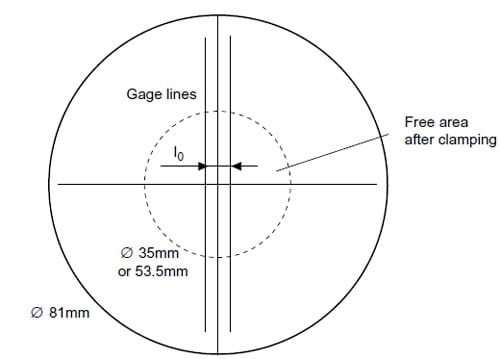
Figure 6: Gage length tracing on a circular sheet
The apparatus used to perform the inflation tests consisted of a circular pressure chamber capped by the test sample and sealed with an annular clamp, Fig.7. Dry compressed air was used as the pressurizing fluid. The base and clamps were machined from6061 aluminum stock. The base included ports for pressure measurements and to admit and vent air. Air inlet control was via a needle valve. Pressure measurements were made with a 0-344 kPa (0-50 psi) pressure transducer for Viton and a precision 0-206 kPa (0-30 psi) Bourdon gage for natural latex and pure gum rubber. Both instruments were calibrated against mercury and water manometers. Both pressure gages could be connected at the same time. A second needle valve was used to deflate the membrane while recording the corresponding stretch ratio response. The entire apparatus was designed to fit on the x-y stage of a Nikon universal measurement microscope.
Two clamp sizes were used for the tests. Natural latex and pure gum rubbers were tested with a clamp allowing for a 35mm diameter free zone. However, due to its low ultimate elongation, Viton required a larger 53.5mm diameter clamp in order to achieve a sufficiently large radius of curvature in the inflated shape. Both clamps were machined with a beveled edge as depicted in Fig.7 to allow for free deformation of the inflated sheet. Belleville spring washers under the clamping bolts proved useful in preventing air leaks over the entire range of pressures. Insufficient clamping forces can allow slipping of the sheet between the clamp and base at high stretch ratios and be a source of experimental errors as noted by Hart-Smith and Crisp [22].
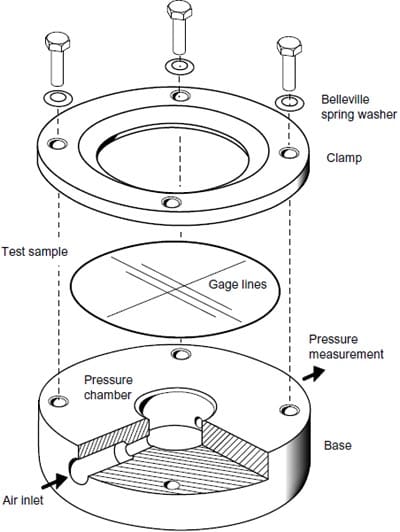
Figure 7: Inflation test apparatus.
As the sample inflates, the original gage length l0 adopts a curved shape, so that direct measurements of the stretched gage length ls not possible. Instead, measurement of
the (x,y,z)coordinates of three points, a, b, and c, indicated in Fig.8 enables first computing the radius of curvature and finally the stretched gage length, ls. The stretch ratio at a given inflation pressure is then:
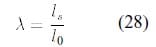
Calculation 28
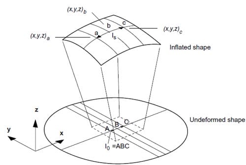
Figure 8: Inflated shape and deformed gage length.
It is not absolutely necessary that the deformed gage length be centered at the pole of the inflated shape. The location of point (x,y,z)bin the neighborhood of the pole is enough to ensure the validity of a biaxial stress state assumption. The ability to track the location of the deformed gage length ls more important. The (x,y,z)coordinates were determined by translating the test apparatus under the microscope objective and focusing the crosshairs on the measurement point. The (x,y)values were obtained to ±1μm resolution from the digital readout of linear encoders attached to the microscope stage. The extremely shallow depth of focus of the microscope allowed z-axis measurements repeatable to within ±0.5μm, as taken from a second digital readout attached to the microscope objective’s rack. All three coordinate values were written simultaneously to a text file through an RS-232 interface. Pressure values were recorded manually when using the 0-206 kPa (0-30 psi.) Bourdon gage and written to a separate text file when employing the 0-344 kPa (0-50 psi.) pressure transducer. The test procedure is summarized below:
- Measure original gage length.
- Admit air.
- Measure coordinates at three points along the gage length.
- Measure pressure.
- Repeat steps 2-4 until the preset maximum pressure.
- Vent air in steps and repeat measurement to assess hysteresis.
Viton exhibited a noticeable viscoelastic behavior, which complicated testing. Upon a step pressurization, the membrane would not immediately assume an equilibrium position. Before making a measurement, it was necessary to wait between 5 and 30 min. depending on the stretch rations.
At high pressures, the gage lines tended to blur due to the separation of the ink particles. This made it difficult to locate measurement points through the microscope. In the case of natural latex, the line blurring problem was exacerbated by membrane thinning at a high stretch ratios. By Eq. 26, the thickness of ts of the latex membrane subjected to the maximum stretch ratio λ1 = λ2 = λ = 4.86 achieved during the test is
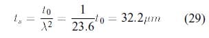
(λ3 = t0 where t0 = 0.762 mm was the original undeformed thickness). At this thickness natural latex becomes almost translucent, reducing the contrast of the gage lines. Changing the microscope magnification from 20 x to 5x, and reducing lighting helped to mitigate the problem.
One of the peculiarities of rubber-like materials is the nonmonotonic form of the measured inflation pressure vs. stretch ratio curve, shown in Fig.9 for natural latex. At a certain value of λ, the addition of air causes the pressure to decrease rather than to increase. The material becomes more compliant and the added air mass is translated into further deformation without raising the internal pressure8. As still more air is added, the internal pressure stabilizes and then starts increasing again, indicating less compliance to deformations. This apparent strain hardening is attributed to crystalization phenomena in rubber-like materials [33]. As shown in Fig.10, Viton did not exhibit pressure stabilization, rather it burst shortly after a slight drop in inflation pressure. The non-monotonicity of the inflation pressure represents an unstable bifurcation behavior9 since more than one stretch ratio is possible for a given inflation pressure [11, 29]. This problem was extensively studied due to its influence on flight prediction of meteorological balloons, Alexander [33] and Needleman [34]. A leak-free test assembly has proven necessary in order to accurately discern the onset of this phenomenon.
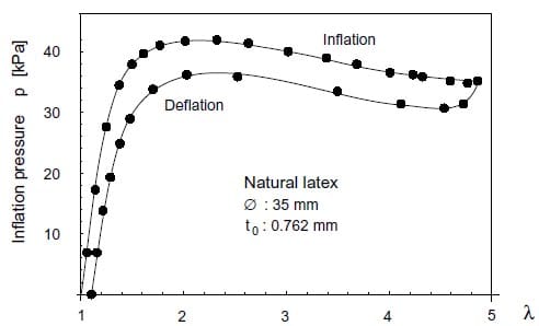
Figure 9: Measured inflation pressure vs. stretch ratio curve for natural latex.
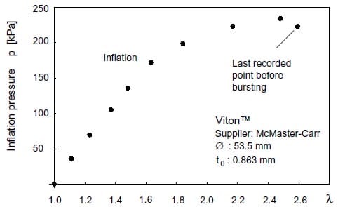
Figure 10: Measured inflation pressure vs. stretch ratio curve for Viton.
3.2 Data Reduction and Calculation of Material Constants
The inflation test yields a series of measurements of grid line mark positions vs. inflation pressure. This data is reduced by the following steps to yield true membrane stress vs. stretch ratios:
- convert coordinate measurements to radii of curvature.
- calculate of deformed gage lengths using radii of curvature and (x,y,z)coordinates.
- calculate stretch ratios.
- calculate the biaxial true (Cauchy) stresses in the neighborhood of the measurement points.
Assuming that the original and deformed gage lengths are coplanar, the radius of curvature r the curve a b c(Fig.11) can be obtained by trigonometric relations as
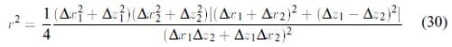
Calculation 30
where all quantities are defined in Fig.11. This was the approach used by Rivlin and Saunders
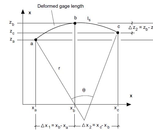
Figure 11: Computation of deformed gage lengths from coordinate measurements.

The true stresses in the neighborhood of the pole of the inflated shape can be found from the well-known expression for the stresses in a membrane under uniform pressure,
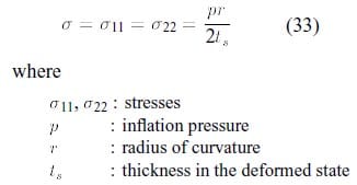
Calculation 33
Except for ts, all quantities on the right hand side of this expression can be measured or computed. By Eq.29, ts is a function of the original thickness and the stretch ratio. The stresses are then
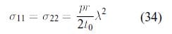
Calculation 34
At this point, the experimental data have been converted into pairs of δ vs. λvalues. A sample plot obtained for pure gum rubber is shown in Fig.12. The next step is to choose a strain energy function and determine the material constants.
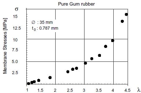
Figure 12: Experimental data points, δ vs. λ for pure gum rubber
We chose the Mooney-Rivlin strain energy function for our study of Viton pads for two main reasons: (a) it is the most commonly used form for which published values are available and (b) the anticipated maximum stretch ratio does not exceed 1.5 for our intended application.
Finding the material constants is a matter of solving an overdetermined system of equations represented by the experimental points. The least squares method provides a means to solve the problem. The usual procedure is to assume any convenient interpolating polynomial and to
calculate the coefficients that minimize the error in fitting the experimental data points such as those indicated in Fig.12. In this case, instead of choosing any function, the analytical expression for the stresses according to Eq.27 is taken as the interpolating function.
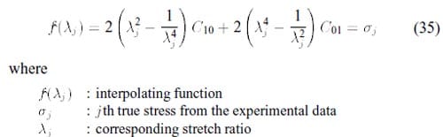
Calculation 35
The unknowns are the Mooney-Rivlin constants C10 and C01. Note that Eq.35 is linear in C10 and C01, which allows the use of a linear least squares procedure (by contrast, Ogden’s strain energy function, Eq.21, is nonlinear in the material constants αi and requires a nonlinear least squares procedure, Twizell and Ogden [35].) The goal is to minimize the following function (see for example, ref.[36] p.258), F(C10;01)=jXn1 [C10’1(
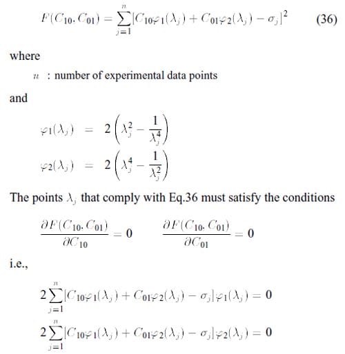
Calculation 36
which can be arranged as a system of two linear equations from which C10 and C01 can be readily obtained,
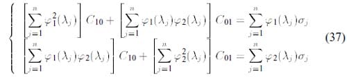
Calculation 37
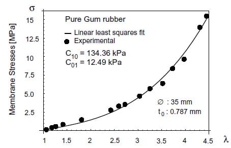
Figure 13: Example of least squares fit of the Mooney-Rivlin form to experimental data.
Kubitza [29] for a similar material. The results are in reasonable agreement in spite of the fact the tests were performed with markedly different specimen sizes.
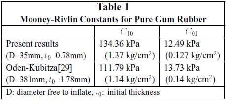
Table 1
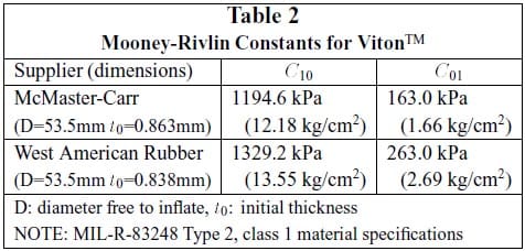
Table 2
Table 2 shows the material constants for MIL-SPEC grade Viton test samples obtained from two different vendors. These values turned out to be considerably higher than the constants for pure gum rubber. A third commercial-grade Viton sample was not tested due to its extremely low elongation at break (estimated at less than 130%) and its chemical susceptibility to the solvent-based marker used to trace the gage lines.
The values for C10 and C01 listed for the first sample of Viton were checked with a simple four-element finite element model of a flat sheet intended to simulate the zone near the pole of the inflated shape (by neglecting again curvature effects). A series of prescribed displacements in two orthogonal directions were imposed in steps to reproduce the values of stretch ratios obtained from the test data. A comparison of the true stress vs. stretch ratio evolution obtained both from the finite element modeling and the experimental data is shown in Fig.14. This simple check served as a qualification of the finite modeling with the experimentally obtained data. The validity of the Mooney-Rivlin constants is of course limited to the loading mode from which they were derived. In the present investigation of a flat pad under compression, these constants are assumed to be valid as long as the deformation remains “as homogeneous as possible.”
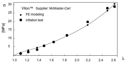
Figure 14: Comparison of experimental data with a finite element model.
4 Finite Element Modeling of the Proposed Shapes
A commercial finite element modeling program, Abaqus v.5-2 [37], was chosen to qualify our experimental results and to evaluate proposed pad designs. Abaqus includes strain energy functions valid for several hyperelastic constitutive models: Mooney-Rivlin’s form (Eq.10), second order deformation form (Eq.15), Ogden’s form (Eq.21).
It also includes the Neo-Hookean form since it can be obtained as a particular case of the Mooney-Rivlin form with C01 =0. Ogden’s strain energy function can be formulated with up to a six term (n=6) approximation of Eq.21. In addition, any of the constitutive models presented previously can be included through a user-defined subroutine (UHYPER).
A Digital Equipment Corporation Alpha AXP-based workstation was used to run all finite element models. Typical CPU times ranged from a few minutes to several hours depending on the loading level and degree of mesh refinement. With the exception of a few simple models, Patran v.3 [38] was used for mesh generation.
4.1 Model Description
The pressure pad problem was modeled with the following assumptions,
- Perfect adhesion of the pad faces to the compressing surfaces (once in contact, the pad faces do not separate). This assumption is usually valid for the high pressure die attach process where one side the pad is held by the rough active surface of the die and the other side is glued to the pressure plate (see Fig.1).
- Constant load applied by the compressing surfaces (as opposed to constant normal tractions).
- Perfect rigidity of the compressing surfaces. This assumption is not strictly valid for the high pressure die attach process in which the adhesive acts as an elastic foundation below the die, Fig.1.
A typical mesh used to model a square pad with a central hole will be used as an example to describe the finite element modeling. A three-dimensional model was adopted since the objective was to study contact stresses and visualize their distribution on the pad faces. Due to the symmetry of the geometry, boundary conditions, and loads, the modeling can be done on one eighth of the actual square pad. The effect of the rest of the pad can bemodeled by imposing the appropriate boundary conditions to the model as indicated in Fig.15. The midsurface nodes are constrained to remain on the same x-y plane at all times during the loading history (when uz displacements occur, these nodes move as a whole, but independent movements in the x and y directions are still possible). Again, by symmetry considerations only one of the rigid compressing surfaces is modeled.
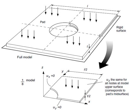
Figure 15: Pressure pad modeling and boundary conditons.

Figure 16: Mesh modeling a pad with a central hole.
Three-dimensional eight-node linear-interpolation mixed-formulation elements were used throughout the modeling (Abaqus element type C3D8H). When necessary, six-node mixedformulation triangular prism elements (Abaqus element type C3D6H) were used as mesh fillers. The use of thesemixed-formulationelementsweremandated by the incompressibility of rubber-like materials for which the stresses cannot be uniquely determined from the displacements 11. Three hundred and ninety 3-D elements were defined for the example in Fig.16. Only three elements were used along the thickness to maintain an adequate aspect ratio in the entiremodel. The height of all elements were the same, but an alternative “pre-distorted” mesh for extremely high loads may consider unequal element heights. Such a mesh is generated in a way that “negates” unfavorable distortions under loads, by making the original element shapes as if they were deformed in the opposite direction.
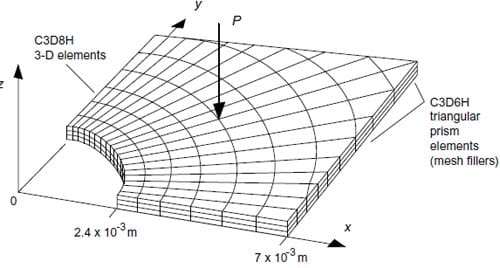
Figure 17: Use of interface elements to detect contact stresses.
A different type of element was used to model the interaction of the lower pad face with the rigid compressing surface. The three dimensional C3D8H elements in the mesh of Fig.17 were overlaid on the l
ower surface with interface elements IRS4 capable of detecting contact with a separately defined rigid surface. The lateral edges were also covered with interface elements to model possible bulging and contact with the rigid surface. However, only two rows of lateral interface elements were defined. The C3D8H elements adjacent to the midsurface of the actual pad (upper surface of the model) did not include them due to the kinematic constraint defined on its constituent nodes (they always remain in the same x-y plane). If interface elements were defined there, the contact force would become undetermined if actual contact occured. Fortunately, extreme lateral bulging was not expected to occur with the loads of the case under study (if it were, the problem could be solved by defining more elements along the thickness). Interface elements also have the ability to deform with the 3-D elements to which they are attached and thus give the true (Cauchy) contact stresses on the rigid surface. The plots shown in the next subsection that describe the distribution of contact stresses are actually describing tractions applied by the rubber pad to the interface elements. Friction between the interface elements and the rigid surface was considered to be infinite (perfect adhesion) but could have been modeled with any values from 0 to infinty.
A concentrated constant load Pwas applied in the -z direction to the upper surface of the mesh (midsurface of the actual pad), Fig.16. This load was automatically considered by Abaqus as uniformly distributed over the entire upper surface due to the kinematic constraint of its nodes (which are prescribed to remain in the same x-y plane).
Themodel depicted in Fig.16 consists of 610 nodes and 592 elements including the interface elements and has an RMS wavefront of 395 after internal optimization performed by Abaqus. The input file corresponding to this example is included in Appendix C, page 47.
4.2 Finite Element Modeling Results
Due to the kinematic constraints imposed by a large friction coefficient, the contact stresses originated by the compression of a solid rubber pad against a rigid surface are nonuniform, as shown in Fig.18(a). This plot was obtained by modeling one eighth of a 14×14 square by 0.8mm thick solid sheet of Viton subjected to uniform compressive tractions of 400 kPa and using the Mooney-Rivlin constants for the first sample material of Table 2 (C10 = 1194.6 kPa, C01 = 163 kPa). The contact stresses have a peak value of 816 kPa at the center of the pad and decrease toward the edges reaching a value of 71.3 kPa at the corners12. The distribution of contact shear stresses in the x-axis direction is also nonuniform as shown in Fig.18(b). In this case there is a sign reversal, with a peak contact shear stress of +85.6 kPa at the right edge and a minimum of -207 kPa along the vertical axis. Note that there are also contact shear stresses in the y-axis direction, whose distribution is the mirror image of Fig.18(b). Therefore, the true peak values differ from these values and must be found pointwise by performing the corresponding transformation. An upper bound on the true peak value is the square root of 2 times the maximum contact shear stress along a given axis. The signs refer to the direction of the contact shear stresses, positive along the +x direction and negative otherwise. At this load, the amount of lateral bulging at the midsurface of the pad is minimal (7.6 x 10 3 mm). The mesh used to model the solid pad is shown in Fig.20. It models one-eighth of the pad and consists of 162 three-dimensional C3D8H elements and 99 IRS4 interface elements. The normal load applied to the upper surface of the model (midsurface of the actual pad) was 19.6 N, which is equivalent to 400 kPa when distributed over the entire model’s surface.
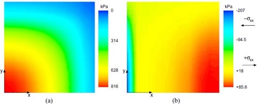
Figure 18: Normal (a) and shear (b) contact stresses applied by a 14 x 14 x 0.8mm solid Viton pad. One-eighth finite element model with a 19.6 N normal load (uniform compressive tractions of 400kPa).
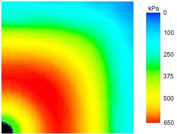
Figure 19: Distribution of normal contact stresses in a 14 x 14 x 0.8mm perforated pad. Hole diameter: 1.2mm. One-eighth finite element model with a 19.6 N normal load.
As noted on page 11, the introduction of a small through hole in the pad relieves the normal contact stresses in its vicinity since the surrounding material is able to deform with relative freedom. If only one hole is placed in the center of the pad while maintaining the same normal load and pad dimensions, the distribution of normal contact stress changes as shown in Fig.19. With a hole of 1.2mm in diameter, the region of peak stresses shifts to a roughly annular zone surrounding the central hole and the maximum value drops 20% to 650 kPa. Note that the normal load applied to the finite element model was the same used for the solid square pad (19.6N) which implies that the average stress is higher than the previous case due to the loss of cross sectional area at the hole. By contrast, the peak values for contact shear stresses increase to +104 kPa and -606 kPa. The finite element model used for this case is similar to the one described in section 4.1. The hole diameter can be increased with a slight reduction of the peak normal contact stress but eventually it begins to increase again due to the effect of the reduced cross sectional area.
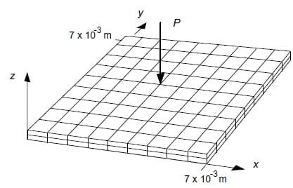
Figure 20: Mesh modeling a solid square pad.
Further reductions in the normal contact stresses can be achievedwith amulti-hole approach. Four holes can be arrayed symmetrically about the center of the pad as indicated in Fig.21. The maximum contact stress with the same normal load decreases to 589 kPa, 28% less than for the original unperforated pad.
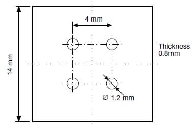
Figure 21: Pad perforated with a symmetrical array of four holes.
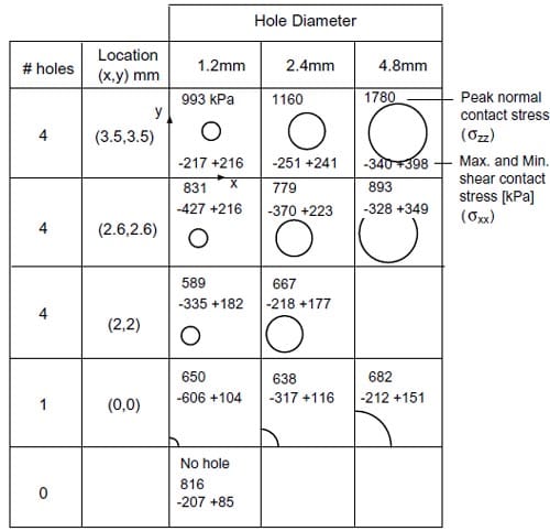
Figure 22: Comparison of peak normal and shear contact stresses for different hole diameters and placement.
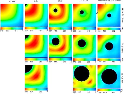
Figure 23: Normal contact stresses for various hole diameters and placement
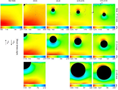
Figure 24: Shear contact stresses for various hole diameters and placement
For a symmetrical four-hole array, the placement as well as the diameters of holes can be changed. Peak normal and shear contact stresses for all cases are summarized in Fig.22. Complete plots for normal and shear contact stresses are shown in Figs.23-24. It is noted that no attempt has been made to consider viscoelastic effects in the finite element modeling. Therefore, the long term values of the peak contact stresses are predicted to fall fromthe values listed in Fig.22 when a viscoelastic constitutive model is included. However, the stress values predicted without considering viscoelasticity are still valid as upper bounds in any given design.
5 Experimental Verification
To verify our finite element modeling of Viton pad deformation and contact stress distribution, and to investigate the effect of interfacial friction, we built a pad test apparatus that allowed direct observation and measuremen
t of samples under a specified load (Fig 25). Like the inflation test apparatus, the entire pad test assembly fit on the calibrated stage of our universal microscope. An air cylinder with a pressure-regulated source supplied the required load. A 0 to 4450 N load cell attached to the piston gave a direct indication of the load. The load cell contacted a ball on the pressure plate assembly, the ball serving to center the load on the sample pad without lateral thrust. A piece of glass was bonded to the pressure plate. The sample pad was then placed on the optically flat surface of the glass. A second piece of glass covered the pad. This 28 mm square x5 mm thick viewing glass was optically flat on both surfaces. It was held in place by a pocket in an aluminumplate with a viewing hole in the center. The pad could be aligned with the center of the assembly by looking through this viewing port and the glass.
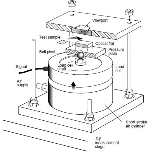
Figure 25: Pad test apparatus.
As the air pressure was turned up and the pad was squeezed, the deformations could be measured through the glass by the microscope and its x,y,z positioning stage.
For some experiments, the contacting surfaces were coated with glycerin to minimize interfacial friction. For others, to approximate a large friction coefficient, the contacting glass surfaces were blasted with aluminumoxide. Prior to grit blasting, the viewing glass wasmasked at 12 places with 0.8 mm wide strips of tape. These strips crossed the pad edge at a right angle, beginning 1mm inside the original pad outline. This minimized the effect of low friction near the measurement location.
Measurements were taken at the corners and at several edge locations while the load was incrementally increased up to roughly 1000N. The bulging edge of the pad was used for the point ofmeasurement in all cases where it could be seen clearly. With a large friction coefficient, the contacted edge of the pad did not move significantly, and visible deformation was limited to edge bulging. For the glycerin cases, the bulge was not significant and therefore, the contacted edge of the pad was measured.
A 15x15x0.86mm Viton pad with a 4.7mm diameter center hole was coated with glycerin, tested with a 890N load, and results compared with a finite element model that assumed a zero friction coefficient. The corners moved 1.89mm, versus the predicted 2.27mm, and the midpoints of the edgesmoved an average of 1.40mmversus the predicted 1.609mm, Fig.26. The central hole shrank approximately 1mm in diameter during the test, while the finite element model predicted a 1.03mm increase in diameter. The agreement within 20% for the edge displacements seemed reasonable since the actual coefficient of friction was certainly larger than zero, as evidenced by the dissimilar behavior at the central hole.
The same test was conducted using the grit blasted glass surfaces with a 1183N load to simulate a large friction coefficient. In this case, the measurements correspond to the outline of the bulging edges. The midpointsmoved an average of 0.252mm versus the 0.141mmpredicted by finite element modeling assuming an infinite friction coefficient. By contrast, the corners exhibit a wide variation between experimental and predicted displacements as shown in Fig.27. The experimental errors were certainly larger in this test due to the small magnitude of the measured displacements and the uncertainty about the value of the actual friction coefficient.
A qualitative test was run to determine the degree of agreement of the finite element model’s normal contact stress results with the actual pads. A “pressure indicating” paper was used to record the normal contact stresses originated by compression of test pads. This paper consists of two coated polyester sheets assembled face-to-face13. The first sheet is coated with a microencapsulated dye and the second with a color developing layer. The microcapsules break in a controlled fashionwhen the film is compressed, leaving an image with intensity proportional to the local pressure. While quantitative measurements are possible with a densitometer, we limited our evaluation to qualitative comparisons. Several film types are offered, we chose the “SL” grade, with a 480-2400 kPa pressure range. The paper was placed between the pad and the viewport. A load of 1000N was applied and photographs taken. Three 14x14x0.8mm square pad designs were tested: pad with no holes, pad with one 2.4mm diameter central hole, and pad with four 1.2mm diameter holes arranged in a 4mm square grid (see Fig.21). The test load was determined to impose average compressive tractions of 5 MPa over the unperforated 14x14mm square pad. The experimental results are shown in Fig.28 and the corresponding finite element results under a 996N load in Fig.29.
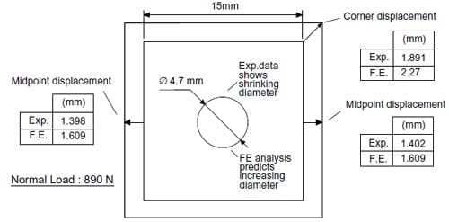
Figure 26: Comparison of experimental and finite element displacements in a perforated Viton pad with glycerin (small friction coefficient)
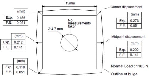
Figure 27: Comparison of experimental and finite element displacements in a perforated Viton pad, large friction coefficient
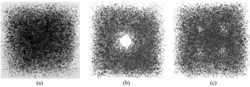
Figure 28: Normal contact stresses registered by a pressure indicating paper on three pad designs. (a) No hole, (b) one 2.4mm diameter hole, and (c) four 1.2mm diameter holes. Normal load: 1000N, pad dimensions: 14 x 14 x 0.86mm, supplier: McMaster-Carr
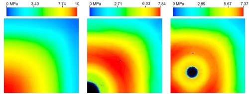
Figure 29: Normal contact stresses from a finite element analysis of the three pad designs of Fig.28. Normal load of 996N in all cases.
Experiment and prediction are in good qualitative agreement. The pad with no holes has normal contact stresses that are high at its center, and very low at the edges. Adding a single center hole shifts the region of normal contact stresses to the surrounding region as predicted by finite element modeling. Low contact stresses are evident next to the edge of the hole. Four holes spread the contact stresses out more uniformly. The edge of the pad has a reasonable value of contact stresses.
6 Conclusions
Elastic properties of gum rubber, natural latex, and Viton were obtained using experimental methods. Inflation tests were conducted to derive material constants for a Mooney-Rivlin constitutive model. This correlated well for modest deformations in the case of Viton. The results were used in a finite element model to evaluate flat, perforated pressure pads for microelectronic applications. Properties of the Viton samples tested varied significantly with supplier.
Using theMooney-Rivlin strain energy function, finite element methods were used to study pad deformations under compression and the corresponding distribution of contact stresses on a rigid surface. A number of competing perforated pad designs were evaluated. For the base case, a solid 14mm square by 0.8mm thick pad, the maximum normal contact stress occurred at the center with a peak value of more than twice the average over the entire pad.
Pad deformations under load were measured optically, compared with the displacements of a finite element model, and found to be in reasonable agreement. Uncertainty of interfacial friction was the largest component of this error. Direct measurements of the pads’ normal contact stress distributions were made using a pressure-indicating film. These tests
showed good qualitative agreement with the finite element modeling.
Judicious perforation of flat pads was found to greatly reduce the variation and maximum value of normal stresses. Our preferred design for a 14 mm square by 0.8 mm thick Viton pad, used four 1.2 mm holes symmetrically arrayed in a 4 mm square grid, centered on the pad (Fig.21). Compared to an unperforated pad, the finite element modeling indicated a 28% reduction in the maximum normal contact stress. However, this reduction was obtained at the expense of an increase in the contact shear stresses. While a great deal of intuition was gained in the course of this work, detailed finite element models are still required to truly optimize pad perforation patterns.
7 Acknowledgments
The authors wish to thank Wayne Mack for his work on the data acquisition equipment, Annie Warren and Colleen Hawk for their efficient system administration, Joel Bartlett for his invaluable contribution on color graphics capture, and Amitabh Srivastava for his aid in formatting this report.
Appendix A
Deformation Measures in Finite Elasticity Theory
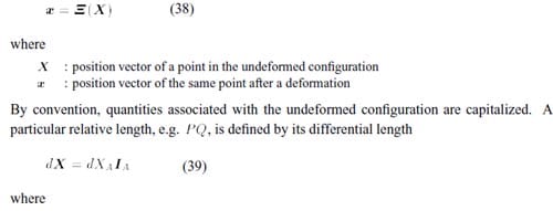
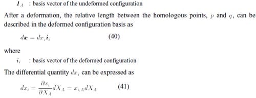
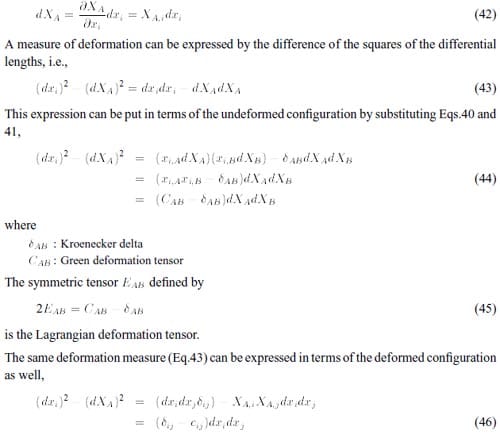
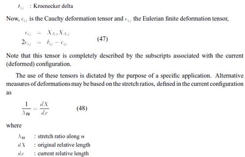
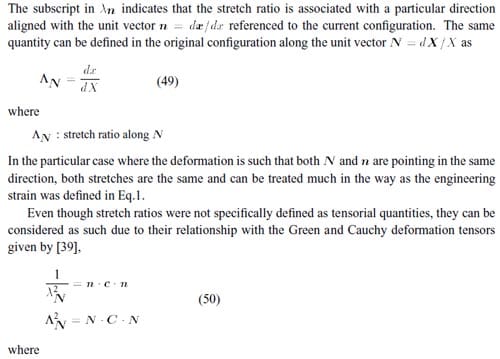
Following is a brief development of deformation and its measures in finite elasticity theory. For a more thorough treatment, see [8, 39]. To derive measures of deformation in finite elasticity, consider a collection of points in an initially unstressed configuration indicated by C0 in Fig.30. After a finite deformation, this same collection of points occupies configuration 1. Points in the two configurations are referenced to different coordinate systems, Xi for the initial state and xi for the deformed state. The description of the deformation will depend on the reference configuration chosen for the analysis. If the Lagrangian description is chosen, the attention is centered on what happens to a point say initially at P. By contrast, the Eulerian description emphasizes what happens at a particular point in space such as p. Both configurations, undeformed and deformed, are related by a mapping between corresponding position vectors that can be expressed as [8, 39]
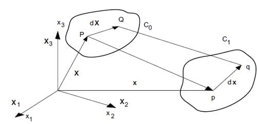
Figure 30: Initial and final configurations

Appendix B
Experimental data and Results
p: inflation pressure, r: radius of curvature, λ: stretch ratio, δ:membrane stress
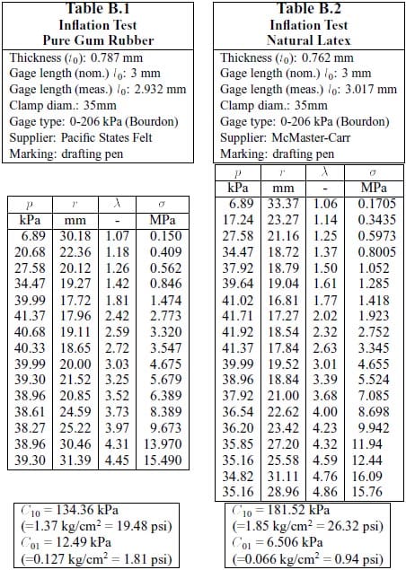
Table B.1 and Table B.2
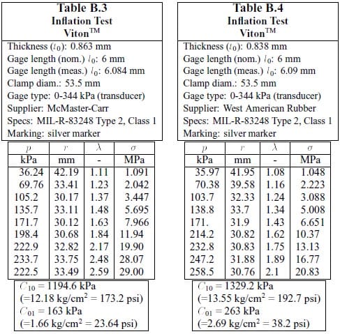
Table B.3 and Table B.4
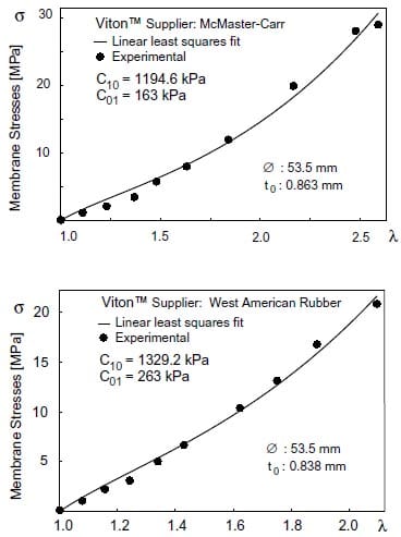
Figure 31: Least squares fit of the experimental data for the tested Viton samples.
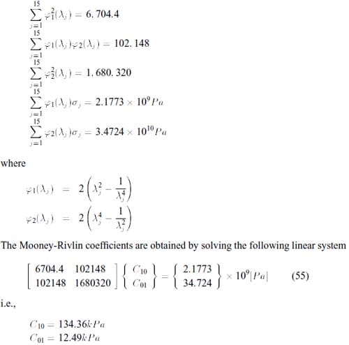
Least Squares Fit Example for Pure Gum Rubber
The least squares fit problem expressed by Eq.37 can be set up for a pure gum rubber test by using the fifteen data points listed in Table B.1:
Appendix C
Sample Abaqus Input File for a Perforated Pad
An Abaqus input file for running a finite element model of a 14x14x0.8mm square pad with a central hole of diameter 4.8mm is shown in the listing on page 48. The numbering scheme for the first layer of nodes is shown in Fig.32, page 52. This input file was generated manually but it could have been obtained with Patran as well. Lines that begin with * indicate Abaqus keywords, while those which begin with ** are comment lines. The rest of the lines are user-defined input values.
The input file is loosely organized into five sections,
- Node definitions.
- Kinematic constraints imposition.
- Element definition.
- Material properties definition.
- Loading imposition and output requests.
No explicit units are indicated in the file, however, all quantities are understood to be expressesd in SI units (dimensions in meters, forces in Newtons, and material constants in Pascals). The results are thus obtained in SI units (stresses in Pascals, displacements in meters).
The analysis has been set up with a 1/8 model of the actual pad due to symmetry considerations. The lower surface of the pad is compressed against a perfectly rigid surface by a concentrated force acting fromabove the midsurface of the model. The nodes in the midsurface are constrained to remain on the same x-y plane with a multipoint constraint imposed with *EQUATION. A dummy node, numbered 1000, is used to formulate this kinematic constraint. The rigid surface is defined with the *RIGID SURFACE keyword which requires additional input to place a local coordinate system and the generator of a plane surface (START and LINE keywords). It is important that the local coordinate system be defined with its third axis “towards” the 3-Dmodel (the normals of the rigid surfaces and elements in the model must have opposite directions). Otherwise, contact will not be detected. Interface elements associated with the lower rigid surface detect the contact stresses produced by the pad’s compression.
A Mooney-Rivlin material with user provided constants is defined with the *HYPERELASTIC, N=1 option (N=2 defines a second order deformation form). Perfect friction (infinite friction coefficient) is indicatedwith *FRICTION,ROUGH,while *SURFACE CONTACT,NO SEPARATION indicates that once an interface element contacts the rigid surface it remains attached to it for the rest of the analysis.
The *STEP keyword initiates the loading definition and output requests. The *NLGEOM option is turned on to indicate the existence of geometric nonlinearities (large deformations). A maximum number of 400 increments (INCR=400) is allowed in the *STEP line and the imposed load is applied according to a ramp function (AMPLITUDE=RAMP).Ramping the load is a requirement for nonlinear cases where convergence of the solution in a given increment may become very difficult to attain.
A “*RESTART” file is written every 5 increments during the analysis. This file allows the user to restart an analysis or to perform post-processing of the final and intermediate results using Abaqus/Post [40]. The results, stresses, their invariants, and the nodal displacements are also written to binary files using the *NODE FILE and *EL FILE keywords (Patran accepts only this file type for post-processing).
Abaqus Input File Listing
*****************************************************************
** FINITE ELEMENT MODELI
NG OF A 14x14x0.8MM SQUARE PERFORATED **
** FLUOROELASTOMER PAD WRL-9/1993 **
** ABAQUS v.5.2-1 **
*****************************************************************
*HEADING
PERFORATED VITON PAD D=4.8MM APPLIED FORCE=-19.6N
**DATA CHECK
*********************
** NODE DEFINITION **
*********************
*NODE,NSET=NX1
81,2.4E-3,0,0
101,3E-3,0,0
121,3.65E-3,0,0
141,4.4E-3,0,0
161,5.2E-3,0,0
181,6E-3,0,0
201,7E-3,0,0
99,0,2.4E-3,0
119,0,3E-3,0
139,0,3.65E-3,0
159,0,4.4E-3,0
179,0,5.2E-3,0
199,0,6E-3,0
219,0,7E-3,0
** NODE ASSOCIATED WITH A RIGID SURFACE
*NODE,NSET=RSURFN
1900,0,0,0
*NGEN,LINE=C,NSET=NX2
81,99,1,1900
101,119,1,1900
121,139,1,1900
141,159,1,1900
161,179,1,1900
181,199,1,1900
201,219,1,1900
*NGEN,LINE=C,NSET=NX2
81,99,1,1900
101,119,1,1900
121,139,1,1900
141,159,1,1900
161,179,1,1900
181,199,1,1900
201,219,1,1900
*NODE,NSET=NX3
202,7E-3,0.6E-3,0
203,7E-3,1.25E-3,0
217,1.25E-3,7E-3,0
218,0.6E-3,7E-3,0
224,7E-3,1.87E-3,0
225,7E-3,2.5E-3,0
226,7E-3,3.25E-3,0
227,7E-3,4.01E-3,0
228,0.00663513,0.00464597,0
229,0.00620496,0.00520658,0
230,0.00572756,0.00572756,0
231,0.00520658,0.00620496,0
232,0.00464597,0.00663513,0
233,4.01E-3,7E-3,0
234,3.25E-3,7E-3,0
235,2.5E-3,7E-3,0
236,1.87E-3,7E-3,0
248,7E-3,4.85E-3,0
249,7E-3,5.8E-3,0
250,6.4E-3,6.4E-3,0
251,5.8E-3,7E-3,0
252,4.85E-3,7E-3,0
270,7E-3,7E-3,0
** DUMMY NODE FOR EQUATION
4000,0,0,0.4E-3
*NCOPY,CHANGE NUMBER=900,OLD SET=NL1,SHIFT,NEW SET=NL4
0,0,0.40E-3
,,,,,,,
*NFILL
NL1,NL4,3,300
*NSET,NSET=XBC,GENERATE
381,501,20
681,801,20
981,1101,20
*NSET,NSET=YBC,GENERATE
399,519,20
699,819,20
999,1119,20
*************************************
** KINEMATIC CONSTRAINT IMPOSITION **
*************************************
*EQUATION
2
NL1,3,1,4000,3,-1
*BOUNDARY
XBC,2
YBC,1
RSURFN,1,6
** RIGID SURFACE DEFINITION
*RIGID SURFACE,TYPE=CYLINDER,ELSET=CONTAC
0,0,0,10E-3,0,0
0,10E-3,0
START,0,0
LINE,9E-3,0
************************
** ELEMENT DEFINITION **
************************
*ELEMENT,TYPE=C3D8H
81,81,101,102,82,381,401,402,382
204,204,224,225,205,504,524,525,505
228,228,248,249,229,528,548,549,529
*ELEMENT,TYPE=C3D6H
203,203,224,204,503,524,504
250,250,270,251,550,570,551
*ELGEN,ELSET=EL1
81,18,1,1,6,20,20,3,300,300
204,12,1,1,3,300,300
228,4,1,1,3,300,300
203,2,24,24,3,300,300
227,2,22,22,3,300,300
250,2,-18,-18,3,300,300
232,2,-16,-16,3,300,300
** INTERFACE ELEMENT DEFINITION (DETECTION OF
** CONTACT WITH RIGID SURFACE)
*ELEMENT,TYPE=IRS4
** LOWER PAD SURFACE 2081,81,101,102,82,1900
2204,204,224,225,205,1900
2228,228,248,249,229,1900
** LATERAL,HOLE
3081,81,381,382,82,1900
** LATERAL,EDGE
3201,201,202,502,501,1900
3203,203,224,524,503,1900
3224,224,225,525,524,1900
3218,219,519,518,218,1900
3236,217,517,536,236,1900
3235,236,536,535,235,1900
*ELEMENT,TYPE=IRS3
2203,203,224,204,1900
2250,250,270,251,1900
*ELGEN,ELSET=CONTAC
** LOWER PAD SURFACE
2081,18,1,1,6,20,20
2204,12,1,1
2228,4,1,1
2203,2,24,24
2227,2,22,22
2250,2,-18,-18
2232,2,-16,-16
** LATERAL,HOLE
3081,18,1,1,2,300,30
** LATERAL,EDGE
3201,2,1,1,2,300,300
3203,2,24,24,2,300,300
3224,3,1,1,2,300,300
3226,2,22,22,2,300,300
3227,2,22,22,2,300,300
3218,2,-1,-1,2,300,300
3236,2,16,16,2,300,300
3235,3,-1,-1,2,300,300
3233,2,18,18,2,300,300
3252,2,18,18,2,300,300
***************************************************
** MATERIAL PROPERTIES DEFINITION, MOONEY-RIVLIN **
** HYPERELASTIC C10=1.194MPa C01=0.163MPa **
***************************************************
*MATERIAL,NAME=VITON
*HYPERELASTIC,N=1
1.194E6,0.163E6
*SOLID SECTION,ELSET=EL1,MATERIAL=VITON
*INTERFACE,ELSET=CONTAC
*FRICTION,ROUGH
*SURFACE CONTACT,NO SEPARATION
***********************************
** LOADING AND OUTPUT DEFINITION **
***********************************
*RESTART,WRITE,FREQUENCY=5
*STEP,NLGEOM,INC=400,AMPLITUDE=RAMP
*STATIC
0.1,1,1E-20,0.1
*CLOAD
1049,3,-19.6
*PRINT,CONTACT=YES
*EL PRINT,ELSET=EL1,POSITION=AVERAGED AT NODES,FREQUENCY=5
S,MISES
E
*EL PRINT,ELSET=CONTAC,POSITION=AVERAGED AT NODES,FREQUENCY=5
S
*NODE PRINT,FREQUENCY=5
U
*NODE FILE
COORD
U
*EL FILE
S,SINV
*END STEP
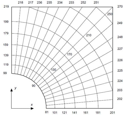
Figure 32: Numbering scheme for the first layer of nodes (z=0).
REFERENCES
- Hamburgen, W., Fitch, J.S., “Packaging a 150-W Bipolar ECL Microprocessor,” IEEE Trans.CHMT, Vol.16, No.1, pp 28-38 (Feb 1993)
- Wessely, H., T¨urk, W., Schmidt, K.H., Nagel, G., “Computer Packaging,” Siemens Forsch.-u. Entwickl.-Ber., Vol.17, No.5, pp.234-239 (1988)
- Wessely, H., “Packaging System for High Performance Computer,” Proc.Sixth IEEE/ CHMT Int.Electronic Manufacturing Technology Symposium, Nara, Japan, Apr.26-28, 1989, pp.83-89, IEEE, NJ (1989)
- Hacke, H.-J., private communication (Oct.1993).
- Du Pont Polymers Inc., “Viton Selection Guide,” Cat.# 226965B, Wilmington, DE 19880-0011 (1992)
- Arnold, R.G., Barney, A.L., Thompson, D.C., “Fluoroelastomers,” Rubber Chem.Tech- nol., Vol.46, No.3, pp.619-651 (1973)
- Treloar, L.R.G., “The Physics of Rubber Elasticity,” Clarendon Press, Oxford (1958)
- Malvern, L.W., “Introduction to the Mechanics of a Continuum Medium,” Prentice-Hall, Englewood Cliffs, N.J. (1969)
- Green, A.E., Adkins, J.E., “Large Elastic Deformations,” Clarendon Press, Oxford, (1970)
- Green, A.E., Zerna, W., “Theoretical Elasticity,” Clarendon Press, Oxford (1968)
- Oden, J.T., “Finite Elements of Nonlinear Continua,” McGraw-Hill, New York (1972)
- Rivlin, R.S., “Large Elastic Deformations of Isotropic Materials IV. Further Developments of the General Theory,” Phil.Trans.Roy.Soc., Vol.A241, No.835, pp.379-397 (Oct.5,1948)
- Mooney, M., “A Theory of Large Elastic Deformation,” J.Appl.Phys, Vol.11, No.9, pp.582-592 (Sep.1940)
- Rivlin, R.S., Saunders, D.W., “Large Elastic Deformations of Isotropic Materials VII. Experiments on the Deformation of Rubber,” Phil.Trans.Roy.Soc., Vol.A243, No.865, pp.251-288 (Apr.24,1951)
- Klosner, J.M., Segal, A., “Mechanical Characterization of a Natural Rubber,” PIBAL Report No.69-42, Dept.ofAerospace Engineering andAppliedMechanics, Polytechnic Institute of Brooklyn (Oct.1969)
- Ishihara, A., Hashitsume, N., Tatibana, M., “Statistical Theory of Rubber-Like Elasticity IV (Two-Dimensional Stretching),” J.Chem.Phys., Vol.19, No.12, pp.1508-1512 (Dec.1951)
- Alexander, H., “AConstitutiveRelation for Rubber-LikeMaterials,” Int.J.Engng.Sci., Vol.6, No.9, pp.549-563 (Sep.1968) [Oden ‘72 p.388]
- James, A.G., Green, A., Simpson, G.M., “Strain Energy Functions of Rubber I. Characterization of Gum Vulcanizates,” J.Appl.Polymer Sci., Vol.19, No.3, pp.2033-2058 (Mar.1975)
- Morman, K.N., Pan, T.Y., “Application of Finite-Element Analysis in the Design of Automotive Elastomeric Components,” Rubber Chem.Technol., Vol.61, No.3, pp.503-533 (Jul.-Aug.1988)
- Yeoh, O.H., “Characterization of Elastic Properties of Carbon-Black-Filled Rubber Vulcanizates,” Rubber Chem.Technol., Vo
l.63, No.5, pp.792-805 (Nov.-Dec.,1990) - Hart-Smith, L.J., “Elasticity Parameters for Finite Deformations of Rubber-like Materials,” Z.angew.Math.Phys., Vol.17, No.5, pp.608-626 (Sep.1966)
- Hart-Smith, L.J., Crisp, J.D.C., “Large Elastic Deformations of Thin Rubber Membranes,” Int.J.Eng.Sci., Vol.5, No.1, pp.1-24 (1967)
- Ogden, R.W., “Large Deformation Isotropic Elasticity – On the Correlation of Theory and Experiment for IncompressibleRubberlike Solids,” Proc.Roy.Soc.Lond.,Vol.A326,No.1567, pp.565-584 (Feb.1972)
- Hall, M.M,“Pressure Distribution over the Flat End Surfaces of Compressed Solid-Rubber Cylinders, J.Strain Analysis, Vol.6, No.1, pp.38-44, (Jan.1971)
- Treloar, L.R.G., “Stresses andBirefringence inRubberSubjected toGeneralHomogeneous Strain,” Proc.Phys.Soc., Vol.60 pt.2, No.338, pp.135-144 (Feb.1,1948)
- Treloar, L.R.G., “Stress-Strain Data for Vulcanised Rubber under Various Types of Deformation,” Trans.Faraday Soc., Vol.40, pp.59-70 (1944)
- Treloar, L.R.G., “Strains in an Inflated Rubber Sheet, and theMechanismof Bursting,” Trans.I.R.I., Vol.19, pp.201-212 (1944)
- Adkins, J.E., Rivlin, R.S., “Large Elastic Deformation of IsotropicMaterials IX. The Deformation of Thin Shells,” Phil.Trans.Roy.Soc., Vol.A244, No.888, pp.66-531 (May 7, 1952)
- Oden, J.T., Kubitza, W.K., “Numerical Analysis of Nonlinear Pneumatic Structures,” Proc. 1st Int. Colloquium on Pneumatic Structures, Stuttgart, May 11-12, 1967, pp.87-107, Technische Hochschule, Stuttgart (1967)
- Finney, R.H., Kumar, A., “Development of Material Constants for Nonlinear Finite-Element Analysis,” Rubber Chem.Technol., Vol.61, No.5, pp.879-891 (Nov-Dec.1988)
- Kong, D., White, J.L., “Inflation Characteristics of Unvulcanized Gum and Compounded Rubber Sheets,” Rubber Chem.Technol., Vol.59, No.2, pp.315-327 (May-Jun.1986)
- ASTM D412-92, “Standard Test Methods for Vulcanized Rubber and Thermoplastic Rubbers and Thermoplastic Elastomers – Tension,” Annual Book of ASTM Standards, Section 9, Vol.09.01, Rubber, Natural and Synthetic – General Test Methods; Carbon Black, American Society for Testing and Materials, Philadelphia (1993)
- Alexander, H., “Tensile Instability of Initially Spherical Balloons,” Int.J.Engng.Sci., Vol.9, No.1, pp.151-162 (Jan.1971)
- Needleman, A., “Inflation of Spherical Rubber Balloons,” Int.J.Solids Struct., Vol.13, No.5, pp.409-421 (1977)
- Twizell, E.H., Ogden, R.W., “Non-linearOptimization of theMaterialConstants inOgden’s Stress- Deformation Function for Incompressible IsotropicElasticMaterials,” J.Austral.Math.Soc., Ser.B., Vol.24, pp.424-434 (1983)
- Atkinson, K.E., “Elementary Numerical Analysis,” J.Wiley & Sons, New York (1985)
- Hibbit, Karlsson, & Sorensen, Inc., “Abaqus/Standard User’s Manual v.5.2,” Vol.I & II, HKS, Pawtucket, RI (1992)
- PDA Engineering, “P3/PATRAN User Manual,” Costa Mesa, CA (1993)
- Mase, G.E., Mase, G.T., “Continuum Mechanics for Engineers,” CRC Press, Boca Raton, FL (1992)
- Hibbit, Karlsson, & Sorensen, Inc., “Abaqus/Post User’s Manual v.5.2,” HKS, Pawtucket, RI (1992)